Introduction to Pandas
MScAS 2025 - DSAS Lecture 3
Ilia Azizi
2025-10-07
Why Pandas?
Core Benefits
- DataFrames & Series for labeled, heterogeneous tabular data
- Built on NumPy : all NumPy benefits plus flexible indexing
- Database-like operations : groupby, merge, pivot, join
- Time series functionality : date/time indexing and resampling
- Missing data handling : robust NaN/None management
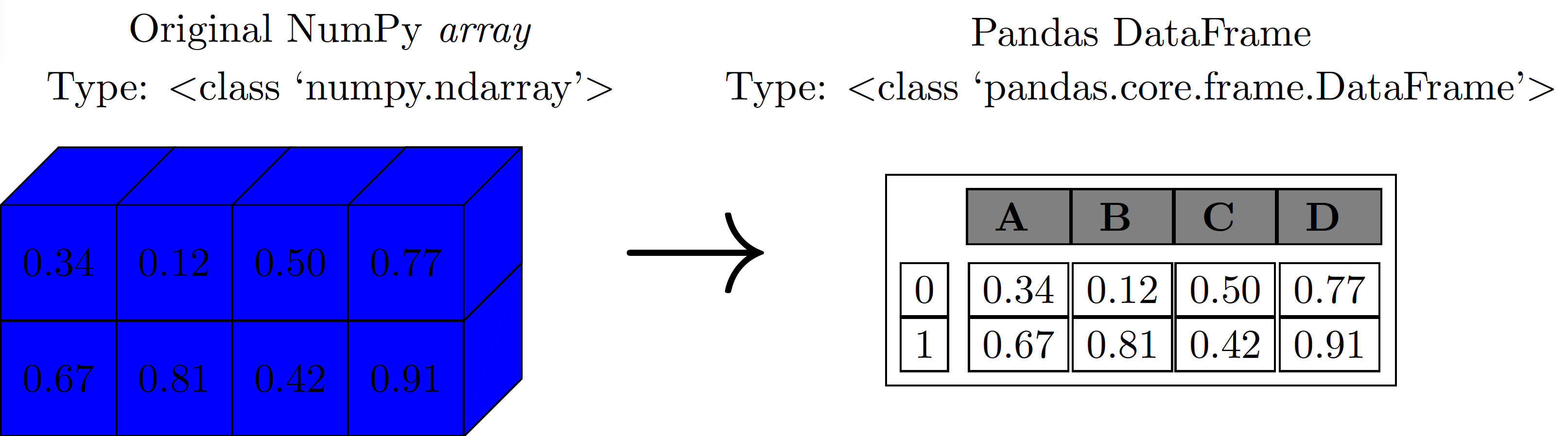
From Arrays to DataFrames
NumPy arrays use positions (0, 1, 2…), while Pandas DataFrames use meaningful labels (PolicyID, date, zone). This makes actuarial data analysis more intuitive and robust!
The Power of Labeled Data
Pandas uses meaningful labels instead of positions. E.g., merge policy data + claims by PolicyID → automatic alignment!
❌ NumPy (Position)
Issues:
- Position-based only
- Sorting breaks links
- Manual matching
✅ Pandas (Labels)
Benefits:
- Auto alignment
- Meaningful names
- Safe operations
🤔 Pop Quiz
The main advantage of Pandas indices over NumPy array is?
- Indices make data load faster
- Indices allow meaningful labels and automatic alignment in operations
- Indices reduce memory usage
- Indices are only useful for time series
Pandas Objects
What is a Series?
A Series is a 1D labeled array capable of holding any data type. Think of it as a column with a name for each row.
What is a DataFrame?
A DataFrame is a 2D labeled data structure with columns of potentially different types.
Key inspection methods
head(n)/tail(n): View first/last n rowsinfo(): Column types, non-null counts, memorydescribe(): Summary statistics (mean, std, quartiles)shape: Dimensions (rows, columns)dtypes: Data type of each columncolumns: Column names
Two Ways to Index: Key Differences
loc: Label-based indexing (slice endpoint inclusive)iloc: Integer position-based indexing (slice endpoint exclusive, like Python slicing)
loc - Label-based:
iloc - Position-based:
🤔 Pop Quiz
What’s the main difference between loc and iloc?
- loc is faster than iloc
- loc uses labels, iloc uses integer positions
- iloc can only select single elements
- loc is for rows, iloc is for columns
Reading Different File Formats
File Types
Pandas supports many file formats. We’ll focus on the most common ones in actuarial practice.
| Format | Function | Delimiter | Common Use |
|---|---|---|---|
| CSV | pd.read_csv() |
Comma (,) |
Claims data, policies |
| TSV/TXT | pd.read_csv(sep='\t') |
Tab/Custom | Legacy systems |
| Excel | pd.read_excel() |
Binary | Spreadsheet reports |
| JSON | pd.read_json() |
Structured | Web APIs, modern apps |
File Paths
Use relative paths from your working directory: 'data/file.csv' or absolute paths: 'C:/Users/name/data/file.csv'. Forward slashes (/) work on all operating systems.
Common parameters for pd.read_csv():
# Custom delimiter
df = pd.read_csv('file.txt', sep=';')  # semicolon-separated

# Skip rows (e.g., skip header comments)
df = pd.read_csv('file.csv', skiprows=3)

# Select specific columns only
df = pd.read_csv('file.csv', usecols=['Claims', 'Payment'])

# Specify data types
df = pd.read_csv('file.csv', dtype={'Zone': str, 'Claims': int})

# Handle missing values
df = pd.read_csv('file.csv', na_values=['NA', 'missing', '-'])

# Set index column
df = pd.read_csv('file.csv', index_col='ID')
Note
Let’s load the Swedish Motor Insurance dataset from the NumPy lecture, a classic actuarial dataset from 1977. The dataset contains the following variables:
- Kilometres: Distance driven per year (1: <1k, 2: 1-15k, 3: 15-20k, 4: 20-25k, 5: >25k)
- Zone: Geographic zone (1: Stockholm/Göteborg/Malmö, 2-7: Other regions)
- Bonus: No-claims bonus (years since last claim + 1)
- Make: Car model (1-8: specific models, 9: all others)
- Insured: Policyholder years (exposure)
- Claims: Number of claims
- Payment: Total claim payments (SEK)
Essential First Steps
After loading data, always inspect its structure, data types, and quality. This helps identify issues early and understand your dataset.
🤔 Pop Quiz
What does pd.read_csv('data.csv', usecols=['Age', 'Premium']) do?
- Skips the ‘Age’ and ‘Premium’ columns
- Loads only the ‘Age’ and ‘Premium’ columns
- Sets ‘Age’ and ‘Premium’ as the index
- Renames columns to ‘Age’ and ‘Premium’
Selection & Filtering
Idea
Use boolean conditions to filter rows based on criteria.
Logical Operators
Combine conditions (each condition must be in parentheses) using:
&for AND|for OR
~for NOT
Matching Against a List of Values
Filter rows where column values match a list of values.
🤔 Pop Quiz
How do you combine multiple conditions in Pandas boolean indexing?
- Use ‘and’ as well as ‘or’
- Use ‘&&’ as well as ‘||’
- Use ‘&’ as well as ‘|’
- Use ‘AND’ as well as ‘OR’
Operations on Data
Key Insights
Like NumPy, Pandas operations are vectorized (fast, no loops needed). Pandas adds two powerful features:
- Index preservation: Labels stay attached to results
- Automatic alignment: Operations align by labels, not position (missing labels →
NaN)
Common operators: + (add()), - (subtract()), * (multiply()), / (divide()), ** (pow())
🤔 Pop Quiz
What happens when you add two Series with different indices?
- An error is raised
- Pandas aligns indices automatically, using NaN for missing index values
- Only matching indices are kept
- Missing values are filled with 0
GroupBy & Aggregation
Note
GroupBy follows three steps: Split data into groups → Apply function → Combine results.
Grouping by Multiple Columns
Pass a list of column names to group by multiple dimensions simultaneously. Result has a MultiIndex. Use .unstack() to pivot into a readable table format.
Applying Multiple Functions at Once
Use .agg() with a list of functions for quick summary statistics, or a dictionary to apply different functions to different columns. Essential for creating comprehensive risk reports!
Two Powerful GroupBy Operations
.transform(): Returns same shape as input, broadcasts group statistics back to original rows (for adding group-level features).filter(): Returns subset of original data, keeps/discards entire groups based on a condition
Transform (add group statistics):
Filter (keep entire groups):
🤔 Pop Quiz
What does df.groupby('Zone')['Claims'].sum() return?
- The original DataFrame with an extra column
- A Series with total claims for each Zone
- A single number (total of all claims)
- A DataFrame with all claims data grouped
Applying Functions
When to use map()
Use map() to replace values in a Series (like “find & replace”). Perfect for converting codes to names (e.g., Zone 1 → “Stockholm”). Works with dictionaries or functions.
Tip
Use apply() for calculations with conditions: if/else logic, multiple columns, custom formulas. Works on Series or DataFrame (with axis=1 for rows).
Note
Use axis=1 when your calculation needs multiple columns from each row (e.g., Claims ÷ Insured).
🤔 Pop Quiz
You want to replace Zone codes (1, 2, 3…) with city names. Which method should you use?
- apply() with axis=1
- transform()
- map() with a dictionary
- groupby()
Time Series
Handling Dates
Convert string dates to datetime objects using pd.to_datetime() for time-based operations.
Setting Datetime as Index
Setting datetime as the index enables powerful time-based slicing and resampling operations (e.g., analyzing claim trends over time).
Tip
Resampling changes the frequency of time series data (e.g., daily → weekly → monthly).
Common Resampling Frequencies
| Alias | Frequency | Example Use |
|---|---|---|
D |
Calendar day | Daily claims |
B |
Business day | Trading days |
W |
Weekly | Weekly reports |
M |
Month end | Monthly summaries |
Q |
Quarter end | Quarterly reports |
A |
Year end | Annual statistics |
🤔 Pop Quiz
Why do we use pd.to_datetime() on date columns?
- To sort dates in ascending order
- To convert string dates into datetime objects for time-based operations
- To format dates for display
- To extract the year from dates
Handling Missing Data
Missing Data Representation
Pandas uses NaN (NumPy) and None (Python) interchangeably for missing data. Both are treated as “missing” by Pandas operations. Common in actuarial datasets (e.g., incomplete claims, pending investigations).
Tip
Use isnull() and notnull() to create boolean masks for filtering missing data. Combine with .any() or .all() to check across rows/columns.
When to Drop Missing Data?
Use dropna() when missing values are truly invalid or represent data collection errors.
⚠️ Caution: Dropping can result in lose of valuable information! Consider the subset parameter to drop only when specific critical columns are missing.
Imputation Strategies
fillna() replaces missing values with meaningful substitutes. Common strategies:
- Constant (0, “Unknown”): When missing = absence
- Mean/Median: For numerical data (preserve distribution)
- Forward/Backward fill: For time series (carry observations forward)
🤔 Pop Quiz
What does fillna(0) do?
- Drops all rows with missing values
- Replaces all NaN values with 0
- Creates a new column filled with zeros
- Fills only the first NaN value with 0
Concatenation
Why Concatenate?
pd.concat() combines multiple DataFrames along an axis. E.g. to combine data from different time periods, regions, or data sources (e.g., merging quarterly claim reports).
Note
axis=0 (default) stacks rows vertically. axis=1 stacks columns horizontally.
Row-wise (axis=0):
Column-wise (axis=1):
Managing Duplicate Indices
By default, concat() preserves original indices, which can create duplicates! Use ignore_index=True to create a clean sequential index (0, 1, 2…).
🤔 Pop Quiz
What does pd.concat([df1, df2]) do by default?
- Combines DataFrames side-by-side (adds columns)
- Stacks DataFrames vertically (adds rows)
- Merges DataFrames based on common columns
- Creates a MultiIndex automatically
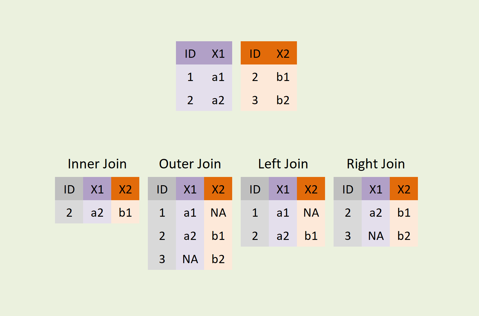
Merge & Join
Join Types: The “What” of the Join
- One-to-One: Each key matches once (e.g., Policy → Customer)
- One-to-Many: Each key matches many (e.g., Zone → Policies)
- Many-to-Many: Multiple matches both sides (use cautiously!)
Join Methods: The “How” of the Join
- Inner: Only matching keys
- Left/right: All from left + matches from right
- Outer: All records from both


Warning
Many-to-Many creates all possible combinations. Result size can explode! Use cautiously.
Sample Data:
Different Join Types:
🤔 Pop Quiz
In a one-to-many merge, what gets duplicated?
- Nothing gets duplicated
- Entries from the “one” side
- Entries from the “many” side
- The merge key
Key Takeaways
Essential concepts covered today:
Pandas Objects : Series & DataFrames with labeled indices for flexible data handling
Data I/O & Inspection :
read_csv(),head(),info(),describe()for loading and exploringSelection & Filtering : Boolean indexing,
loc/iloc,isin()for targeted subsettingIndex Alignment : Automatic label matching during operations (NaN for missing indices)
GroupBy Operations : Split-apply-combine for category-wise aggregations and risk segmentation
Custom Functions :
apply()andmap()for actuarial calculations (risk scores, severity)Time Series :
to_datetime(), DatetimeIndex, andresample()for temporal analysisMissing Data :
isnull(),dropna(),fillna()for handling incomplete actuarial dataCombining Data :
concat()andmerge()for joining policy, claims, and customer datasets
Topics NOT covered today (see lecture notes for details)
- Hierarchical indexing (MultiIndex) : For multi-dimensional data (Zone × Product × Time)
- Pivot tables : Excel-like cross-tabulations and summary reports
- Broadcasting : DataFrame-Series operations with axis control
- Advanced index alignment : Custom fill values and alignment strategies
- Data reshaping :
stack(),unstack(),melt(), andpivot()operations (the latter two will be added tomorrow)
📚 Resources: Pandas lecture notes for comprehensive coverage and more examples
Questions?
![]()
DSAS 2025 | HEC Lausanne