3 Modeling the spread of COVID-19 in a single country
3.1 The logistic model in R
Using the filtered dataset, we study the spread of COVID-19 with the logistic model. Letting \(C_{i}(t) = C_{d_{0,i} + t,i}\), the model for country \(i\) can be expressed as:
\[ C_{i}(t) = \frac{K_{i} \cdot C_{i}(0)}{C_{i}(0) + (K_{i}-C_{i}(0)) \, \exp(-R_{i}\,t)} \]
The goal is to find the final number of cases \(K_{i}\) and the infection rate \(R_{i}\). We implement this in R using the following function:
# here, we assume that data is a data frame with two variables
#  - t: the number of event days
#  - confirmed: the number of confirmed cases at time t
logistic_model <- function(data) {
  data <- data %>% arrange(t)
  C_0 <- data$confirmed[1]
  C_max <- data$confirmed[nrow(data)]
  nls(
    formula = confirmed ~ K / (1 + ((K - C_0) / C_0) * exp(-R * t)),
    data = data,
    start = list(K = 2 * C_max, R = 0.5),
    control = nls.control(minFactor = 1e-6, maxiter = 100)
  )
}
Notice:
- We use the nonlinear least square method
stats::nlsto fit the unknown parameters. - In R, the formula above is
confirmed ~ K / (1 + ((K - C_0)/C_0) * exp(-R * t)). - As starting point \((K_0, R_0)\) for the optimiser, we set \(R_0 = 0.5\) and \(K_0 = 2 \, C(t^*)\), where \(t^*\) is the latest information about accumulated confirmed cases.
- We further set the
controlargument asnls.control(minFactor = 1e-6, maxiter = 100).
3.2 The logistic model applied to data from Switzerland
From covid19_data_filtered, extract a table covid19_ch which corresponds to data for Switzerland.
Then:
- We use the function above to fit the logistic model for Switzerland
- We describe its output (fitted parameters,
broom::tidy()might be useful here) - We discuss the goodness-of-fit.
- We plot the fitted curve, as well as observed data points.
- And finally, we present the predictions of the model. What is the estimated final size of the epidemic and infection rate in Switzerland?
We will start by presenting the data we own for the model we want to describe.
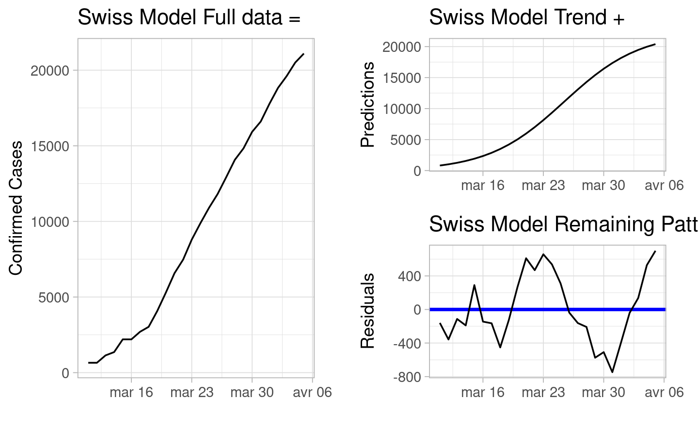
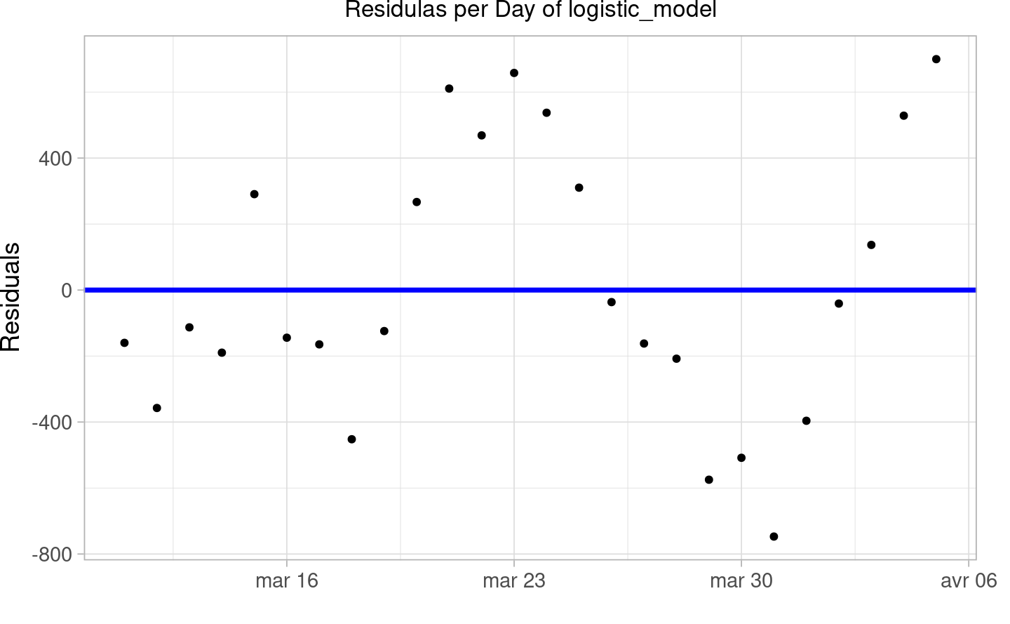
Comment: In general we can see that there is an increasing trend for the confirmed cases of COVID-19 in Switzerland (which does not come as a surprise). The trend seems to follow quite well the pace of the observations, and the residuals seems to focus around zero, with some variation, especially towards the end of March.
| term | estimate | std.error | statistic | p.value |
|---|---|---|---|---|
| K | 22253.429 | 345.696 | 64.4 | 0 |
| R | 0.227 | 0.002 | 96.3 | 0 |
Comment: we can see that the two parameters found are both statistically significant and both positively correlated to the independent variable.
Now, we will discuss the goodness of fit of the model by comparing it to a null model having the confirmed case explained by a constant variable.
#>
#> Call:
#> glm(formula = confirmed ~ 1, data = covid19_ch)
#>
#> Coefficients:
#>             Estimate Std. Error t value   Pr(>|t|)
#> (Intercept)     9650       1370    7.04 0.00000022 ***
#> ---
#> Signif. codes:  0 '***' 0.001 '**' 0.01 '*' 0.05 '.' 0.1 ' ' 1
#>
#> (Dispersion parameter for gaussian family taken to be 48822367)
#>
#>     Null deviance: 1220559163  on 25  degrees of freedom
#> Residual deviance: 1220559163  on 25  degrees of freedom
#> AIC: 537.1
#>
#> Number of Fisher Scoring iterations: 2
#> Analysis of Variance Table
#>
#> Model 1: confirmed ~ K/(1 + ((K - C_0)/C_0) * exp(-R * t))
#> Model 2: confirmed ~ 1
#>   Res.Df Res.Sum Sq Df      Sum Sq F value              Pr(>F)
#> 1     24    4200305
#> 2     25 1220559163 -1 -1216358858    6950 <0.0000000000000002 ***
#> ---
#> Signif. codes: 0 '***' 0.001 '**' 0.01 '*' 0.05 '.' 0.1 ' ' 1We then plot the fitted curve and the observations.
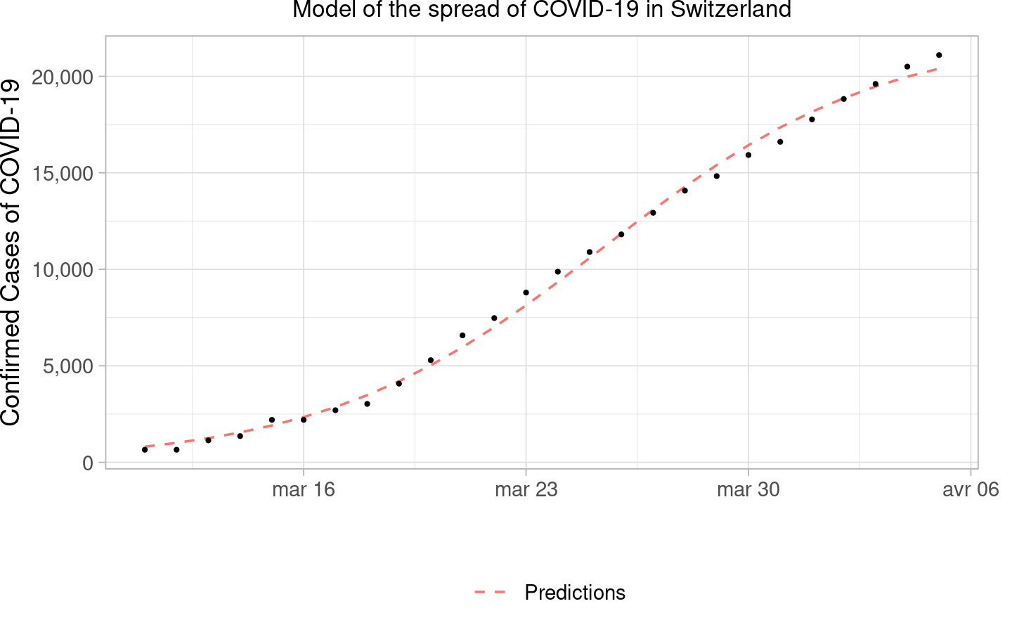
Comment: As we can see the predictions are following quite well the observations, meaning that the model is working quite well. However, it is woth mentioning that the model is fitted on the whole datasets, which could lead to some form of overfitting, not having a separation in training and test set, meaning that once dealing with new data, the prediction ability of the model could decrease quite a lot.
Eventually, the prediction the estimated final size of the epidemic and infection rate in Switzerland is 20400.238.