8 Modelling

In this last chapter we will move on to the modelling part of our analysis, in order to get to the point in which we can answer our research questions, hoping to be able to confirm what has already be found in the different exploratory data analysis in the previous chapters.

To be able to best interpret our results and to have data that could be statistically significant, some corrections have to be done. More specifically we decided to create 4 different variables, namely:

The weekday binary variable: taking value 1 if the day was on the weekend or on a holiday and value 0 otherwise;
The december binary variable: taking value 1 if the date was in December, and 0 otherwise;
The peaktime binary variable: taking value 1 if the time was between 8am and 5pm and 0 otherwise;
The speed_limit_above_25 binary variable: taking value 1 if the speed limits was above 25 and 0 otherwise.

Furthermore, we decided to ignore the WT01 weather variable because it is too general, we prefer to have a clear understanding on what is influencing the results and hence concentrate our efforts on the analysis of well defined variables, such as the rain, the snow and the average wind.

Regarding the response variable, it will be a different one according to the different scenarios. Hence, we will use different variables to answer our initial research questions. What will always be the case is the logistic modelling,all of them being binary.

We then created two different dataframes, one having the weather variables as factors and the other having them as dummies, as already mentioned in the weather EDA, to see wich one of the two performs better, since the factors levels have been decided based only on one year data they are not fully reliable.

We will the follow this process in order to answer all the research questions:

Process
1. Balance the dataframes according to the dependent variable (often being zero-infalted data)
2. Create training and test sets (75% and 25%)
3. Run a regression tree to select the contributing factors
4. Train the models on the training set using a generalized linear model (glm)
5. Create the predicitons using the glm
6. Test the models’ predicitons with the test set and compare them
7. Answer the research question

It has to be noted that the point 3 (hence the selection of the contributing factors) was about to be done using a lasso regression, however, due to a long computational time, limited processes, low computation capabilities and a lack of knowledge of the method by our part, it has been discarded and replaced by a simpler and more familiar regression tree model. However, the code can still be found in the appendix.

We will now move on with our analysis and we will start by modelling the first question.

8.1 Research Question 1

Are deaths lower in roads with speed limit of 25 MPH speed limit relative to the 30 and 40 MPH counterparts? New York City believes “Pedestrians struck by vehicles traveling at 25 MPH are half as likely to die as those struck at 30 MPH” and although we don’t have experimental data to test the statement under laboratory conditions, we can test whether having 25 vs 30 mph speed limit has actually helped in reducing fatalities by half or not.

Here, we will use the deaths (persons_killed) as dependent variable, so that we can assess its predictability, especially analyzing the correlation with respect to the speed limit (speed_limit_above_25) and how is the value of the latter influencing the predictions former. Especially, we want to see if the predictability of a fatality would double once the speed limit is above 25mph.

8.1.1 First Model: weather variables as factors

As already mentioned, we will start by balancing the dataset, being the output variable zero-infalted, and hence it will result that the best way to forecast it is just to predict zero all the time and have a high sensitivy and a low specifity.

#> Proportion of positives after ubOver : 0.58 % of 189897 observations

We will then proceed with the creation of a test set (25% of the data) and a training set (the remaining 75%).

We then run the regression tree model for the first dataset, having the persons_killed as dependent variable and selecting the weather variables as factors.

#> 
#> Classification tree:
#> rpart(formula = persons_killed ~ ., data = training.set, parms = list(split = "speed_limit_above_25"), 
#>     control = rpart.control(minsplit = 2, minbucket = 1, cp = 0.001))
#> 
#> Variables actually used in tree construction:
#>  [1] aggressive_driving_road     alcohol_involvement        
#>  [3] awnd                        backing_unsafely           
#>  [5] december                    driver_inexperience        
#>  [7] driverless_runaway_vehicle  failure_to_yield           
#>  [9] illnes                      lost_consciousness         
#> [11] multiple_cars               other_lighting_defects     
#> [13] other_vehicular             passing_or_lane            
#> [15] peaktime                    pedestrian_bicyclist_other 
#> [17] prcp                        snow                       
#> [19] speed_limit_above_25        traffic_control_disregarded
#> [21] turning_improperly          unsafe_speed               
#> [23] weekend                    
#> 
#> Root node error: 848/142186 = 0.006
#> 
#> n= 142186 
#> 
#>       CP nsplit rel error xerror xstd
#> 1  0.006      0       1.0    1.0 0.03
#> 2  0.004      3       1.0    1.0 0.03
#> 3  0.003      4       1.0    1.0 0.03
#> 4  0.002      7       1.0    1.0 0.03
#> 5  0.002     10       1.0    1.0 0.03
#> 6  0.002     12       1.0    1.0 0.03
#> 7  0.001     27       0.9    1.0 0.03
#> 8  0.001     33       0.9    1.0 0.03
#> 9  0.001     43       0.9    1.0 0.03
#> 10 0.001     48       0.9    0.9 0.03
#> 11 0.001     72       0.9    0.9 0.03
#> 12 0.001     81       0.9    0.9 0.03
#> [1] 0.98
#> 
#> Classification tree:
#> rpart(formula = persons_killed ~ ., data = training.set, parms = list(split = "speed_limit_above_25"), 
#>     control = rpart.control(minsplit = 2, minbucket = 1, cp = 0.001))
#> 
#> Variables actually used in tree construction:
#> [1] awnd                       illnes                    
#> [3] multiple_cars              pedestrian_bicyclist_other
#> [5] prcp                       unsafe_speed              
#> 
#> Root node error: 848/142186 = 0.006
#> 
#> n= 142186 
#> 
#>      CP nsplit rel error xerror xstd
#> 1 0.006      0         1      1 0.03
#> 2 0.004      3         1      1 0.03
#> 3 0.003      4         1      1 0.03
#> 4 0.002      7         1      1 0.03
#> # A tibble: 12 x 2
#>    value var                           
#>    <dbl> <chr>                         
#>  1 21.0  illnes                        
#>  2 13.7  multiple_cars                 
#>  3 13.0  awnd                          
#>  4  8.55 unsafe_speed                  
#>  5  7.95 prcp                          
#>  6  6.30 pedestrian_bicyclist_other    
#>  7  5.38 peaktime                      
#>  8  4.31 driver_inattention_distraction
#>  9  4.31 speed_limit_above_25          
#> 10  2.53 snow                          
#> 11  2.32 december                      
#> 12  2.15 weekend

Here, by using the control factor of the code for the regression tree, we force the variable speed_limit_above_25 to be one of the decision variables, being the one that we want to control for as the cause of deaths in car crashes. Also, we want the model to have a number of splits higher than two. We run the first regression tree, we select its lowest xerror (0.94636) and we add to it its xstd (0.033491), which gives us the level that we will use (0.979851) to find the CP, notably being the first xerror lower than the level found (which is the tree corresponding to nsplit = 7 and a CP of 0.0023838). We insert this value for the pruning as the cp factor, and we get the resulting tree. It has to be noted that in our case, however, the goal is to find the importance of the variables, which can be found in the last table shown. We can see that the most important variables here are the multiple_cars, the illness and the weather variables (more specifically prcp, and awnd). It is interesting to note the the speed_limit_above_25 is in the top ten most important variables.

We move on by training the glm model on the training set, using only the most important variables by the regression tree, so that we can have a lighter model and, hopefully, more precise.

Table 8.1: RQ1: Summary of glm_model
term	estimate	std.error	statistic	p.value	significance	percentage
(Intercept)	-4.26	0.11	-38.03	0.00	***	0.01
illnes	4.19	0.20	21.30	0.00	***	0.99
multiple_cars	-1.73	0.07	-23.75	0.00	***	0.15
awndlight	1.44	0.43	3.32	0.00	***	0.81
awndmoderate	0.21	0.11	1.92	0.05	.	0.55
awndheavy	0.22	0.11	1.97	0.05		0.56
unsafe_speed	2.27	0.11	20.62	0.00	***	0.91
prcplight	-0.23	0.10	-2.18	0.03		0.44
prcpmoderate	-0.24	0.15	-1.63	0.10		0.44
prcpheavy	-0.03	0.10	-0.26	0.79		0.49
pedestrian_bicyclist_other	2.03	0.17	12.27	0.00	***	0.88
peaktime	-0.54	0.07	-7.52	0.00	***	0.37
driver_inattention_distraction	-0.09	0.09	-1.01	0.31		0.48
speed_limit_above_25	0.23	0.10	2.42	0.02		0.56
snowlight	1.38	0.23	6.04	0.00	***	0.80
snowmoderate	-0.16	0.40	-0.41	0.68		0.46
snowheavy	0.06	0.27	0.22	0.83		0.51
december	0.07	0.13	0.52	0.60		0.52
weekend	0.20	0.08	2.56	0.01		0.55

Table 8.1: RQ1: glm_model diagnostic
null.deviance	df.null	logLik	AIC	BIC	deviance	df.residual	nobs
10378	142185	-4486	9010	9198	8972	142167	142186

The variables that are found to be not significant in the prediction of the persons_killed variable for the first model are, interestingly, quite a lot. While the few that are significant (illnes, unsafe_speed, lost_consciousness, multiple_cars, peaktime, pedestrian_bicyclist_other, speed_limit_above_25 and weekend) are quite infleuncing, having a coefficient quite high. The speed_limit_above_25 is significant at 0.01 % and it has a positive influence on the prediction of the fatalities in a car crash. However, it is not possible to affirm that the probablity doubles, since the coefficient of the glm is not as straightforward to interpret as it could be the one for a simple linear regression. This coefficient represents by how much the log of the odds (indeed it is called log-odd coefficient) of an event increases with an increase of one unit of the corresponding explanatory variable. In our case the coefficient is equal to 0.231. We can transform it back to the probability by taking the

\[\displaystyle \frac{exp(b)}{(1 + exp(b))}\]

with b as the coefficient, which gives 0.557. As we can see, the probability of having a fatality when the speed limit raises above 25 does not double, but it does increase by quite a lot. Those for the others coefficients can be found in the last column of the table above.

We will use the Akaike Information Criterion (AIC) to compare the models, which is a score for models taking the following formula: \[AIC = 2k * 2l \]

k being the number of parameters and l the loglikelihood of the model.

Here, the AIC for this model is 8063.358.

Moreover, to assess the goodness of fit of our model, we run the predictions and we will compare it to the test set. Eventually, we will use the result to compare this model with the following one, which uses the weather variables as dummies.

8.1.2 Second model: weather as dummy variables.

We start by creating the dataframe, which is only modificating the weather variables and put them into dummies, taking value 1 when it was respectively windy, snowy or rainy and 0 otherwise.

Once again we balance the dataset, to avoid the problems abovementioned.

#> Proportion of positives after ubOver : 0.58 % of 189897 observations

And with the balanced dataset we create the test and the training sets (once againg respectively with 25% and 75% of the data).

Now that we are setup, we can run the regression tree model to select the most important variables, again by forcing more than 2 splits and having one of the decision variables the one in which we are interested, i.e. speed_limit_above_25.

#> 
#> Classification tree:
#> rpart(formula = persons_killed ~ ., data = training.set.dummies, 
#>     parms = list(split = "speed_limit_above_25"), control = rpart.control(minsplit = 2, 
#>         minbucket = 1, cp = 0.001))
#> 
#> Variables actually used in tree construction:
#>  [1] alcohol_involvement         awnd                       
#>  [3] backing_unsafely            december                   
#>  [5] failure_to_yield            illnes                     
#>  [7] lost_consciousness          multiple_cars              
#>  [9] other_lighting_defects      passing_or_lane            
#> [11] peaktime                    pedestrian_bicyclist_other 
#> [13] prcp                        snow                       
#> [15] speed_limit_above_25        traffic_control_disregarded
#> [17] unsafe_speed                weekend                    
#> 
#> Root node error: 814/142472 = 0.006
#> 
#> n= 142472 
#> 
#>      CP nsplit rel error xerror xstd
#> 1 0.003      0       1.0      1 0.03
#> 2 0.002      8       1.0      1 0.03
#> 3 0.002     18       1.0      1 0.03
#> 4 0.001     21       0.9      1 0.03
#> 5 0.001     33       0.9      1 0.03
#> 6 0.001     40       0.9      1 0.03
#> [1] 0.987
#> 
#> Classification tree:
#> rpart(formula = persons_killed ~ ., data = training.set.dummies, 
#>     parms = list(split = "speed_limit_above_25"), control = rpart.control(minsplit = 2, 
#>         minbucket = 1, cp = 0.001))
#> 
#> Variables actually used in tree construction:
#>  [1] alcohol_involvement        awnd                      
#>  [3] december                   illnes                    
#>  [5] lost_consciousness         multiple_cars             
#>  [7] other_lighting_defects     peaktime                  
#>  [9] pedestrian_bicyclist_other prcp                      
#> [11] snow                       speed_limit_above_25      
#> [13] unsafe_speed               weekend                   
#> 
#> Root node error: 814/142472 = 0.006
#> 
#> n= 142472 
#> 
#>      CP nsplit rel error xerror xstd
#> 1 0.003      0         1      1 0.03
#> 2 0.002      8         1      1 0.03
#> 3 0.002     18         1      1 0.03
#> # A tibble: 17 x 2
#>       value var                           
#>       <dbl> <chr>                         
#>  1 18.8     speed_limit_above_25          
#>  2 14.8     multiple_cars                 
#>  3 14.2     illnes                        
#>  4 13.1     prcp                          
#>  5 12.3     unsafe_speed                  
#>  6  9.88    awnd                          
#>  7  8.17    lost_consciousness            
#>  8  7.47    driver_inattention_distraction
#>  9  7.42    peaktime                      
#> 10  7.32    weekend                       
#> 11  5.71    alcohol_involvement           
#> 12  5.12    pedestrian_bicyclist_other    
#> 13  5.11    december                      
#> 14  4.58    snow                          
#> 15  2.26    other_lighting_defects        
#> 16  0.00743 pavement_defective            
#> 17  0.00594 animals_action

Here, we follow the same process for pruning as we did before. We get to the resulting tree having its variables’ importances, and we find that speed_limit_above_25 is at the 3rd place, which is pretty interesting and in line with what we are expecting.

Table 8.2: RQ1: Summary of glm_model_dummies
term	estimate	std.error	statistic	p.value	significance	percentage
(Intercept)	-4.39	0.11	-38.41	0.00	***	0.01
speed_limit_above_25	0.16	0.10	1.63	0.10		0.54
multiple_cars	-1.78	0.08	-23.75	0.00	***	0.14
illnes	4.08	0.21	19.03	0.00	***	0.98
prcp1	-0.16	0.08	-2.10	0.04		0.46
unsafe_speed	2.55	0.11	24.23	0.00	***	0.93
awnd1	0.15	0.10	1.47	0.14		0.54
lost_consciousness	3.30	0.26	12.84	0.00	***	0.96
driver_inattention_distraction	-0.13	0.10	-1.28	0.20		0.47
peaktime	-0.50	0.08	-6.72	0.00	***	0.38
weekend	0.33	0.08	4.36	0.00	***	0.58
alcohol_involvement	1.40	0.19	7.35	0.00	***	0.80
pedestrian_bicyclist_other	1.99	0.18	11.34	0.00	***	0.88
december	0.32	0.12	2.81	0.00	**	0.58
snow1	0.43	0.17	2.46	0.01		0.61
other_lighting_defects	4.15	0.65	6.37	0.00	***	0.98
pavement_defective	-11.73	182.53	-0.06	0.95		0.00
animals_action	-11.87	197.02	-0.06	0.95		0.00

Table 8.2: RQ1: glm_model dummies diagnostic
null.deviance	df.null	logLik	AIC	BIC	deviance	df.residual	nobs
10032	142471	-4222	8481	8658	8445	142454	142472

For the second model, the variables that are not significant are quite a lot! Is interesting to note that, even though we have already run a variable selection, there are so many variables that are still not important for the prediction of the fatalities. What is comforting is the fact that the one in which we are interested it is significant, and at a 0.01% level. The coefficient is equal to 0.16. Once again to see the real change in the probability of the fatalities, we have transform the log-odd. Eventually, we get 0.54. Once again, we can say that the probability of a fatality is indeed influenced by the speed of the accident, but we cannot confirm that it does double once the speed limit is above 25mph.

Here the AIC of the model is 8254.703, which compared to the previous one (8063.358), is a bit worse, meaning that we should use the first model to have a better goodness-of-fit.

As already mentioned, we will also use the predictions to compare the two models.

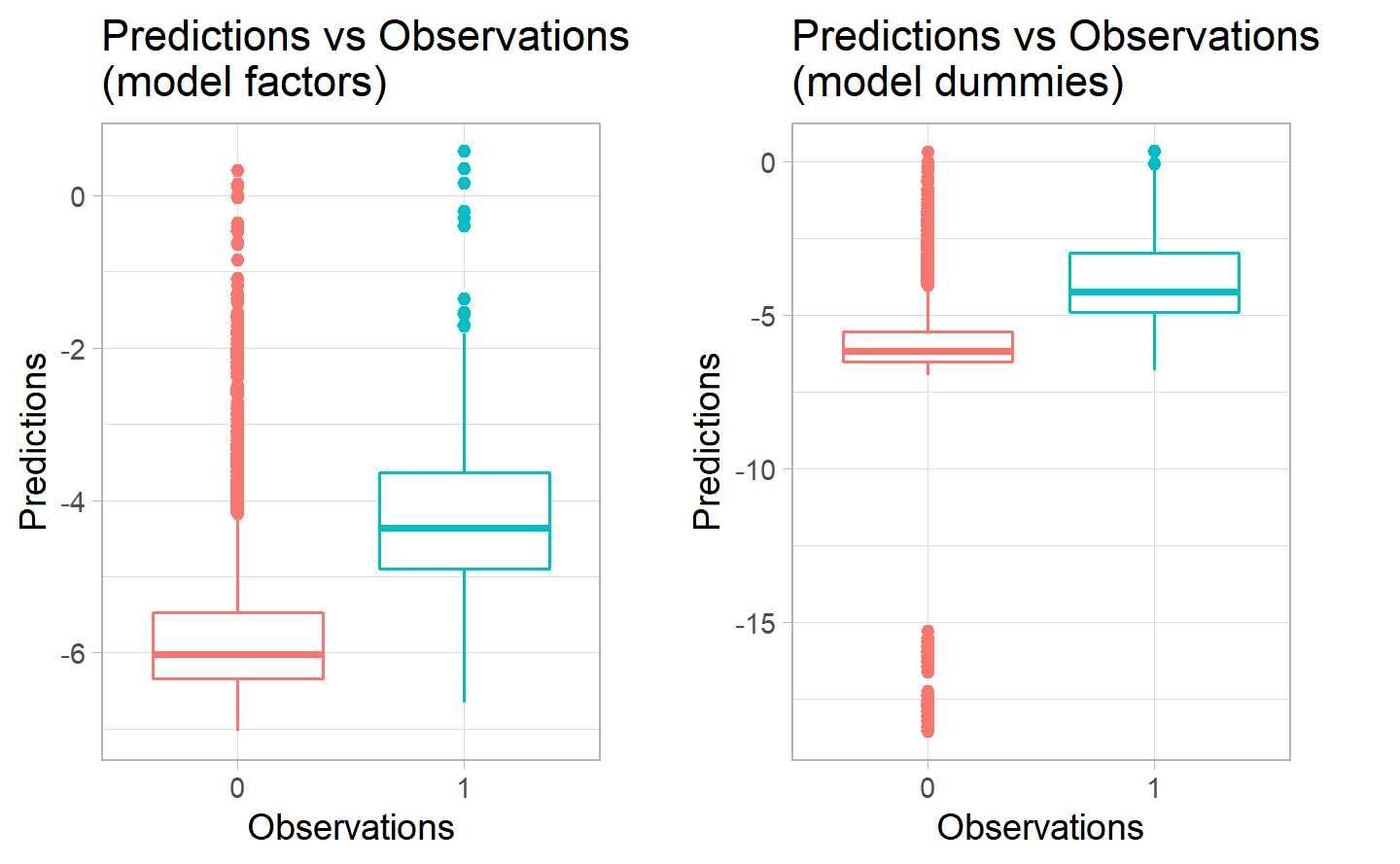
Thanks to the boxplots we can see that actually the two models are performing pretty similarly, which means that they are both performing quite poorly. We can see the the median of the two models for both category is below 0. Moreover, there is a huge variation in both models for the prediciton of the negative category, and a very low variation for the prediction of the positive one, meaning that probably most of the forecast will be equal to 0. This is in line with the dataset, since, before balancing it, we had a very low amount of instances in which there was a positive number for the fatalities. More research on the reasons of fatalities in car crashes has to be done.

8.2 Research Question 2

Do weather conditions (e.g. heavy rain, snow and average wind speed) have a notable influence on wether the accidents will involve multiple car or only one car.

Here we will use the variable multiple_cars that we have previously created, which is taking value 1 when the accident was involving more than a car, and 0 otherwise (see the chapter on EDA collisions for more details).

8.2.1 First model: weather variables as factors

#> Max number of times allowed to replicate minority class is 3 
#>  taking as many samples as the majority class 
#> Proportion of positives after ubOver : 50 % of 296968 observations

Then, we will create the training and test set.

And now we are good to go, so we will run the regression tree that will give us the most important variables to be included in the glm.

#> 
#> Classification tree:
#> rpart(formula = multiple_cars ~ ., data = training.set, parms = list(split = c("prcp", 
#>     "snow", "awnd")), control = rpart.control(minsplit = 2, minbucket = 1, 
#>     cp = 0.001))
#> 
#> Variables actually used in tree construction:
#>  [1] backing_unsafely               driver_inattention_distraction
#>  [3] driver_inexperience            failure_to_yield              
#>  [5] following_too_closely          oversized_vehicle             
#>  [7] passing_or_lane                passing_too_closely           
#>  [9] persons_injured                reaction_to_uninvolved        
#> [11] speed_limit_above_25           traffic_control_disregarded   
#> [13] turning_improperly             unsafe_lane_changing          
#> [15] view_obstructed_limited       
#> 
#> Root node error: 1e+05/222578 = 0.5
#> 
#> n= 222578 
#> 
#>       CP nsplit rel error xerror  xstd
#> 1  0.100      0       1.0    1.0 0.002
#> 2  0.029      2       0.8    0.8 0.002
#> 3  0.021      3       0.8    0.8 0.002
#> 4  0.018      6       0.7    0.7 0.002
#> 5  0.017      7       0.7    0.7 0.002
#> 6  0.014      8       0.7    0.7 0.002
#> 7  0.006      9       0.7    0.7 0.002
#> 8  0.006     10       0.6    0.6 0.002
#> 9  0.006     11       0.6    0.6 0.002
#> 10 0.005     12       0.6    0.6 0.002
#> 11 0.003     13       0.6    0.6 0.002
#> 12 0.002     14       0.6    0.6 0.002
#> 13 0.002     15       0.6    0.6 0.002
#> 14 0.001     19       0.6    0.6 0.002
#> [1] 0.612
#> 
#> Classification tree:
#> rpart(formula = multiple_cars ~ ., data = training.set, parms = list(split = c("prcp", 
#>     "snow", "awnd")), control = rpart.control(minsplit = 2, minbucket = 1, 
#>     cp = 0.001))
#> 
#> Variables actually used in tree construction:
#>  [1] backing_unsafely               driver_inattention_distraction
#>  [3] driver_inexperience            failure_to_yield              
#>  [5] following_too_closely          oversized_vehicle             
#>  [7] passing_or_lane                passing_too_closely           
#>  [9] persons_injured                reaction_to_uninvolved        
#> [11] speed_limit_above_25           traffic_control_disregarded   
#> [13] turning_improperly             unsafe_lane_changing          
#> [15] view_obstructed_limited       
#> 
#> Root node error: 1e+05/222578 = 0.5
#> 
#> n= 222578 
#> 
#>       CP nsplit rel error xerror  xstd
#> 1  0.100      0       1.0    1.0 0.002
#> 2  0.029      2       0.8    0.8 0.002
#> 3  0.021      3       0.8    0.8 0.002
#> 4  0.018      6       0.7    0.7 0.002
#> 5  0.017      7       0.7    0.7 0.002
#> 6  0.014      8       0.7    0.7 0.002
#> 7  0.006      9       0.7    0.7 0.002
#> 8  0.006     10       0.6    0.6 0.002
#> 9  0.006     11       0.6    0.6 0.002
#> 10 0.005     12       0.6    0.6 0.002
#> 11 0.003     13       0.6    0.6 0.002
#> 12 0.002     14       0.6    0.6 0.002
#> 13 0.002     15       0.6    0.6 0.002
#> 14 0.001     19       0.6    0.6 0.002
#> # A tibble: 21 x 2
#>    value var                           
#>    <dbl> <chr>                         
#>  1 3867. following_too_closely         
#>  2 2660. driver_inattention_distraction
#>  3 2364. persons_injured               
#>  4 2137. failure_to_yield              
#>  5 1639. unsafe_lane_changing          
#>  6 1196. backing_unsafely              
#>  7 1180. passing_or_lane               
#>  8 1056. turning_improperly            
#>  9  866. traffic_control_disregarded   
#> 10  358. driver_inexperience           
#> # ... with 11 more rows

Here we can see that by pruning, we get to the point in which the most important variables in the prediction of the involvement of multiple cars in the case of a car crash are following_too_closely, driver_inattention_distraction, persons_injured and failure_to_yield, the rest can be found in the above table. Regarding the weather variables, we can see they are at the bottom. They are probably considered by the model only because it was forced by the coding that has been done. What has to be noted is that, in this case, the pruning of the tree does not seem to be really useful, since the resulting tree has still 23 split and its root node is almost 50%. This suggests that it may not be a good model, and possibly, since they are at the bottom of the table, as already mentioned, the weather variables are not very important for the prediction of the involvement of multiple cars in a car crash.

Subsequently, we will run the glm, to confirm this first hypothesis.

Table 8.3: RQ2: Summary of glm_model
term	estimate	std.error	statistic	p.value	significance	percentage
(Intercept)	0.76	0.01	57.00	0.00	***	0.68
following_too_closely	-2.41	0.02	-98.82	0.00	***	0.08
driver_inattention_distraction	-1.28	0.01	-111.14	0.00	***	0.22
persons_injured	0.81	0.01	71.22	0.00	***	0.69
failure_to_yield	-1.19	0.02	-65.47	0.00	***	0.23
unsafe_lane_changing	-2.30	0.04	-57.23	0.00	***	0.09
backing_unsafely	-1.25	0.02	-55.41	0.00	***	0.22
passing_or_lane	-1.33	0.02	-55.23	0.00	***	0.21
turning_improperly	-1.87	0.04	-49.86	0.00	***	0.13
traffic_control_disregarded	-2.02	0.04	-47.21	0.00	***	0.12
driver_inexperience	-1.19	0.04	-32.25	0.00	***	0.23
passing_too_closely	-0.71	0.02	-32.85	0.00	***	0.33
reaction_to_uninvolved	-1.09	0.04	-26.88	0.00	***	0.25
speed_limit_above_25	-0.45	0.01	-30.53	0.00	***	0.39
view_obstructed_limited	-1.04	0.05	-22.26	0.00	***	0.26
oversized_vehicle	-1.26	0.06	-20.74	0.00	***	0.22
pedestrian_bicyclist_other	-0.43	0.05	-7.99	0.00	***	0.39
lost_consciousness	-1.16	0.12	-9.33	0.00	***	0.24
illnes	-0.83	0.13	-6.25	0.00	***	0.30
glare	-0.92	0.11	-8.65	0.00	***	0.29
outside_car_distraction	-1.23	0.10	-12.06	0.00	***	0.23
tire_failure_inadequate	-0.48	0.12	-4.07	0.00	***	0.38
prcplight	0.03	0.01	2.17	0.03		0.51
prcpmoderate	0.04	0.02	2.38	0.02		0.51
prcpheavy	0.09	0.01	6.61	0.00	***	0.52
awndlight	-0.23	0.09	-2.47	0.01		0.44
awndmoderate	-0.10	0.01	-7.86	0.00	***	0.47
awndheavy	-0.05	0.01	-3.80	0.00	***	0.49
snowlight	-0.03	0.05	-0.74	0.46		0.49
snowmoderate	0.04	0.04	0.83	0.41		0.51
snowheavy	0.16	0.04	4.40	0.00	***	0.54

Table 8.3: RQ2: glm_model diagnostic
null.deviance	df.null	logLik	AIC	BIC	deviance	df.residual	nobs
308559	222577	-135579	271221	271541	271159	222547	222578

From the table, we can see that the all selected variables seem to be important, but the first two levels of snow and rain (light and moderate). This does not come as a surprise, on the contrary is pretty straightforward, as the driving conditions worsen with snow or rain, and only a light or moderate amount of it could not be really influencing. For the significant ones, the coeffients are respectively 0.16 for heavy snow, 0.044 for moderate rain and 0.087 for heavy rain, while for wind -0.234 for the light level (significant at 5%), -0.105 for the moderate level and -0.053 (both significant at 0.01%). Which gives an influence on the probability of having a multiple cars accident of 0.54 for the snow, 0.511 and 0.522 for, respectively, the moderate and heavy rain and 0.442, 0.474 and 0.487 for the light, moderate and heavy wind speed.

So, we can see that the snow seems to have the highest influence on the increase of probability of multiple cars crashes (almost 55%), but only at the heavy level, the rain has almost the same influence on the two levels which are significant, namely moderate and heavy (with an increase around 50%), and the wind is the one with the lowest influence (never reaches the 50%), but it’s also the only one having the three levels significant. However, one could argue that this is due to the fact that in NYC it is almost everyday windy, so it is not actually an influencing factor.

The AIC of this model is 269267.4.

Now we will run the predictions and we will move on to the second model for this question.

8.2.2 Second model: weather dummies

Here, we follow the same process as before, but with the second dataframe, the one with the weather variables as dummies.

So, we start by balancing the dataset.

#> Max number of times allowed to replicate minority class is 3 
#>  taking as many samples as the majority class 
#> Proportion of positives after ubOver : 50 % of 296968 observations

Then, we create the training and the test set with the balanced data.

Subsequently, we can run the regression tree to select the most important variables, by forcing the weather in one of the nodes.

#> 
#> Classification tree:
#> rpart(formula = multiple_cars ~ ., data = training.set.dummies, 
#>     parms = list(split = c("prcp", "snow", "awnd")), control = rpart.control(minsplit = 2, 
#>         minbucket = 1, cp = 0.001))
#> 
#> Variables actually used in tree construction:
#>  [1] backing_unsafely               driver_inattention_distraction
#>  [3] driver_inexperience            failure_to_yield              
#>  [5] following_too_closely          oversized_vehicle             
#>  [7] passing_or_lane                passing_too_closely           
#>  [9] persons_injured                reaction_to_uninvolved        
#> [11] speed_limit_above_25           traffic_control_disregarded   
#> [13] turning_improperly             unsafe_lane_changing          
#> [15] view_obstructed_limited       
#> 
#> Root node error: 1e+05/222578 = 0.5
#> 
#> n= 222578 
#> 
#>       CP nsplit rel error xerror  xstd
#> 1  0.100      0       1.0    1.0 0.002
#> 2  0.029      2       0.8    0.8 0.002
#> 3  0.021      3       0.8    0.8 0.002
#> 4  0.018      6       0.7    0.7 0.002
#> 5  0.017      7       0.7    0.7 0.002
#> 6  0.014      8       0.7    0.7 0.002
#> 7  0.006      9       0.7    0.7 0.002
#> 8  0.006     10       0.6    0.6 0.002
#> 9  0.006     11       0.6    0.6 0.002
#> 10 0.005     12       0.6    0.6 0.002
#> 11 0.003     13       0.6    0.6 0.002
#> 12 0.002     14       0.6    0.6 0.002
#> 13 0.002     15       0.6    0.6 0.002
#> 14 0.001     19       0.6    0.6 0.002
#> [1] 0.612
#> 
#> Classification tree:
#> rpart(formula = multiple_cars ~ ., data = training.set.dummies, 
#>     parms = list(split = c("prcp", "snow", "awnd")), control = rpart.control(minsplit = 2, 
#>         minbucket = 1, cp = 0.001))
#> 
#> Variables actually used in tree construction:
#>  [1] backing_unsafely               driver_inattention_distraction
#>  [3] driver_inexperience            failure_to_yield              
#>  [5] following_too_closely          oversized_vehicle             
#>  [7] passing_or_lane                passing_too_closely           
#>  [9] persons_injured                reaction_to_uninvolved        
#> [11] speed_limit_above_25           traffic_control_disregarded   
#> [13] turning_improperly             unsafe_lane_changing          
#> [15] view_obstructed_limited       
#> 
#> Root node error: 1e+05/222578 = 0.5
#> 
#> n= 222578 
#> 
#>       CP nsplit rel error xerror  xstd
#> 1  0.100      0       1.0    1.0 0.002
#> 2  0.029      2       0.8    0.8 0.002
#> 3  0.021      3       0.8    0.8 0.002
#> 4  0.018      6       0.7    0.7 0.002
#> 5  0.017      7       0.7    0.7 0.002
#> 6  0.014      8       0.7    0.7 0.002
#> 7  0.006      9       0.7    0.7 0.002
#> 8  0.006     10       0.6    0.6 0.002
#> 9  0.006     11       0.6    0.6 0.002
#> 10 0.005     12       0.6    0.6 0.002
#> 11 0.003     13       0.6    0.6 0.002
#> 12 0.002     14       0.6    0.6 0.002
#> 13 0.002     15       0.6    0.6 0.002
#> 14 0.001     19       0.6    0.6 0.002
#> # A tibble: 21 x 2
#>    value var                           
#>    <dbl> <chr>                         
#>  1 3867. following_too_closely         
#>  2 2660. driver_inattention_distraction
#>  3 2364. persons_injured               
#>  4 2137. failure_to_yield              
#>  5 1639. unsafe_lane_changing          
#>  6 1196. backing_unsafely              
#>  7 1180. passing_or_lane               
#>  8 1056. turning_improperly            
#>  9  866. traffic_control_disregarded   
#> 10  358. driver_inexperience           
#> # ... with 11 more rows

Once again, we can see that the pruning of this tree is not really helping, since the results is still quite extensive, with a lot of nodes. What is actually important, is to see that the importance of the weather data seems to be really low for this model, not making the cut for the pruning.

Using the selected variables, we are ready now to run the glm, so that we can assess the importance of weather on the involvement of multiple cars in a car crash. What has to be noted is the fact that we are forcing the selection of the weather variables in the dataset we will use to run the glm, as they are the variables in which we interested in terms of relationship with multiple_cars.

Table 8.4: RQ2: Summary of glm_model_dummies
term	estimate	std.error	statistic	significance	percentage
(Intercept)	0.76	0.01	57.25	***	0.68
following_too_closely	-2.42	0.02	-98.87	***	0.08
driver_inattention_distraction	-1.28	0.01	-111.20	***	0.22
persons_injured	0.81	0.01	71.28	***	0.69
failure_to_yield	-1.19	0.02	-65.45	***	0.23
unsafe_lane_changing	-2.30	0.04	-57.24	***	0.09
backing_unsafely	-1.25	0.02	-55.48	***	0.22
passing_or_lane	-1.33	0.02	-55.29	***	0.21
turning_improperly	-1.88	0.04	-49.88	***	0.13
traffic_control_disregarded	-2.02	0.04	-47.20	***	0.12
driver_inexperience	-1.19	0.04	-32.27	***	0.23
passing_too_closely	-0.71	0.02	-32.95	***	0.33
reaction_to_uninvolved	-1.09	0.04	-26.85	***	0.25
speed_limit_above_25	-0.45	0.01	-30.47	***	0.39
view_obstructed_limited	-1.04	0.05	-22.25	***	0.26
oversized_vehicle	-1.26	0.06	-20.78	***	0.22
pedestrian_bicyclist_other	-0.43	0.05	-8.04	***	0.39
lost_consciousness	-1.16	0.12	-9.38	***	0.24
illnes	-0.83	0.13	-6.25	***	0.30
glare	-0.92	0.11	-8.65	***	0.29
outside_car_distraction	-1.23	0.10	-12.08	***	0.23
tire_failure_inadequate	-0.48	0.12	-4.09	***	0.38
prcp1	0.06	0.01	5.75	***	0.51
awnd1	-0.09	0.01	-6.89	***	0.48
snow1	0.08	0.02	3.22	**	0.52

Table 8.4: RQ2: glm_model_dummies diagnostic
null.deviance	df.null	logLik	AIC	BIC	deviance	df.residual	nobs
308559	222577	-135612	271274	271531	271224	222553	222578

Here, surprisingly, all the variables are significant! Apparently, the glm and the regression tree are not on the same page regarding the imporance of the weather variables. In any case, we can see that the coefficients for the three variables are respectively 0.056, -0.086 and 0.08 for rain, wind and snow. Which means that, when there is rain, in general, the probability of having a multiple car accident increases by 0.514, 0.479 for wind and 0.52 for snow. Once again snow is the one having the highest increase of probability, followed by rain and then wind, which is in line with the previous model. The comment about the wind variable holds also for this situation.

The AIC of the model is 269335.4, which compared to the previous one (269267.4), is slightly worse, meaning that we should go, in theory, for the first model. However, one could argue that, being the difference in AIC so small, and being this model a bit more simple, since it does not need any measurement of the wind, snow and rain, but just an obervation on wether they happened on a given day or not, it could be worth it to have a slightly higher AIC, but for a simpler model.

Now we can compare the predictions.

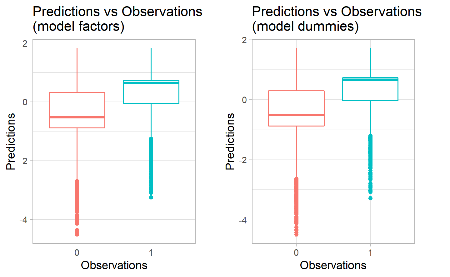
Once again the predictions boxplot are quite similar for the two models, here they seem to be performing a bit better than before. We can see that the average for the second one is slightly higher for the positive category, while, for the negative category, they have a very similar distribution of the predicitons. In both cases there are quite a lot of outliers in the bottom part for both the positive and negative categories. The boxplots do not lead us to a preference of a model over the other.

8.3 Research Question 3

Can we estimate the probability of an injury of an accident using all our variables: Weather, reason of the accident provided by the police from previous cases (contributing factors) and lastly the speed limits.

Here we will use the persons_injured as dependent variable, to analyze, in general, which are the most important variables for the former to be postive. In other words, what are the inlfuencing factors for an injury to happen in a car crash.

8.3.1 First model: weather variables as factors

Once again we create a new balanced dataset, to avoid having an almost perfect sensitivity and very bad specificity, since having a majority of 0 values would make the model mostly out 0 as the prediction, as already explained. So, we want to create a dataset having the same number of observations having injueries and not having any.

#> Max number of times allowed to replicate minority class is 3 
#>  taking as many samples as the majority class 
#> Proportion of positives after ubOver : 50 % of 297084 observations

Then we move on to the creation of training and test set.

And eventually the regression tree to have a first selection of the most important variables. We run it also for this question primarly for two motives: (1) it will make our glm lighter and easier to interpet, avoiding redundancy and the consideration of useless variables that would not be significant, and (2), we can see if there is a consistency within the variable selected by the regression tree and the singificant variables of the glm.

#> 
#> Classification tree:
#> rpart(formula = persons_injured ~ ., data = training.set, control = rpart.control(minsplit = 2, 
#>     minbucket = 1, cp = 0.001))
#> 
#> Variables actually used in tree construction:
#>  [1] alcohol_involvement         awnd                       
#>  [3] backing_unsafely            failure_to_yield           
#>  [5] following_too_closely       lost_consciousness         
#>  [7] multiple_cars               passing_too_closely        
#>  [9] peaktime                    pedestrian_bicyclist_other 
#> [11] speed_limit_above_25        traffic_control_disregarded
#> [13] unsafe_lane_changing        unsafe_speed               
#> 
#> Root node error: 1e+05/222668 = 0.5
#> 
#> n= 222668 
#> 
#>       CP nsplit rel error xerror  xstd
#> 1  0.116      0       1.0    1.0 0.002
#> 2  0.007      1       0.9    0.9 0.002
#> 3  0.007      6       0.8    0.8 0.002
#> 4  0.005      9       0.8    0.8 0.002
#> 5  0.004     10       0.8    0.8 0.002
#> 6  0.003     12       0.8    0.8 0.002
#> 7  0.002     13       0.8    0.8 0.002
#> 8  0.002     14       0.8    0.8 0.002
#> 9  0.001     16       0.8    0.8 0.002
#> 10 0.001     17       0.8    0.8 0.002
#> [1] 0.794
#> 
#> Classification tree:
#> rpart(formula = persons_injured ~ ., data = training.set, control = rpart.control(minsplit = 2, 
#>     minbucket = 1, cp = 0.001))
#> 
#> Variables actually used in tree construction:
#>  [1] alcohol_involvement         awnd                       
#>  [3] backing_unsafely            failure_to_yield           
#>  [5] following_too_closely       lost_consciousness         
#>  [7] multiple_cars               passing_too_closely        
#>  [9] peaktime                    pedestrian_bicyclist_other 
#> [11] speed_limit_above_25        traffic_control_disregarded
#> [13] unsafe_lane_changing        unsafe_speed               
#> 
#> Root node error: 1e+05/222668 = 0.5
#> 
#> n= 222668 
#> 
#>       CP nsplit rel error xerror  xstd
#> 1  0.116      0       1.0    1.0 0.002
#> 2  0.007      1       0.9    0.9 0.002
#> 3  0.007      6       0.8    0.8 0.002
#> 4  0.005      9       0.8    0.8 0.002
#> 5  0.004     10       0.8    0.8 0.002
#> 6  0.003     12       0.8    0.8 0.002
#> 7  0.002     13       0.8    0.8 0.002
#> 8  0.002     14       0.8    0.8 0.002
#> 9  0.001     16       0.8    0.8 0.002
#> 10 0.001     17       0.8    0.8 0.002
#> # A tibble: 24 x 2
#>    value var                        
#>    <dbl> <chr>                      
#>  1 2115. multiple_cars              
#>  2 1866. failure_to_yield           
#>  3 1603. passing_too_closely        
#>  4 1410. backing_unsafely           
#>  5  681. traffic_control_disregarded
#>  6  493. pedestrian_bicyclist_other 
#>  7  461. unsafe_speed               
#>  8  282. peaktime                   
#>  9  180. following_too_closely      
#> 10  137. lost_consciousness         
#> # ... with 14 more rows

The most important variables to predict the event of an injury in a car crash appears to be multiple_cars, failure_to_yield, passing_too_closely, backing_unsafely and traffic_control_disregarded. The rest can be found in the above table. However, we can see that in this case the pruning is not very effective, as the selection of the variable is quite large.

Let’s now run the glm to see if it does a better job in understanding which are the most important variables.

Table 8.5: RQ3: Summary of glm_model
term	estimate	std.error	statistic	p.value	significance	percentage
multiple_cars	-0.69	0.01	-65.15	0.00	***	0.33
failure_to_yield	0.82	0.02	51.94	0.00	***	0.69
passing_too_closely	-1.43	0.03	-45.96	0.00	***	0.19
traffic_control_disregarded	1.27	0.03	39.37	0.00	***	0.78
backing_unsafely	-0.91	0.03	-36.33	0.00	***	0.29
pedestrian_bicyclist_other	2.33	0.07	34.69	0.00	***	0.91
unsafe_speed	0.90	0.03	27.37	0.00	***	0.71
peaktime	-0.24	0.01	-26.46	0.00	***	0.44
(Intercept)	0.38	0.01	25.62	0.00	***	0.59
following_too_closely	0.30	0.02	19.91	0.00	***	0.58
speed_limit_above_25	0.22	0.01	17.42	0.00	***	0.55
unsafe_lane_changing	-0.44	0.03	-15.80	0.00	***	0.39
lost_consciousness	2.90	0.19	15.13	0.00	***	0.95
awndmoderate	0.20	0.01	15.08	0.00	***	0.55
awndheavy	0.19	0.01	13.90	0.00	***	0.55
alcohol_involvement	0.54	0.04	13.35	0.00	***	0.63
fell_asleep	0.65	0.08	8.46	0.00	***	0.66
drugs_illegal	1.39	0.17	8.08	0.00	***	0.80
animals_action	-0.75	0.16	-4.81	0.00	***	0.32
snowheavy	-0.12	0.04	-3.26	0.00	**	0.47
snowmoderate	-0.08	0.04	-2.02	0.04		0.48
awndlight	0.14	0.09	1.58	0.11		0.53
pavement_defective	0.18	0.13	1.47	0.14		0.55
using_on_board	0.60	0.45	1.34	0.18		0.65
steering_failure	0.09	0.11	0.85	0.40		0.52
snowlight	0.03	0.04	0.78	0.43		0.51
headlights_defective	0.34	0.47	0.73	0.46		0.58
windshield_inadequate	0.47	1.25	0.37	0.71		0.61
tire_failure_inadequate	-0.01	0.12	-0.12	0.91		0.50

Table 8.5: RQ3: glm_model diagnostic
null.deviance	df.null	logLik	AIC	BIC	deviance	df.residual	nobs
308682	222667	-144518	289095	289394	289037	222639	222668

The variables that are not significant are tire_failure_inadequate, steering_failure, headlights_defective, windshield_inadequate and shoulders_defective_improper. The ones with the highest coefficients are lost_consciousness (2.9), pedestrian_bicyclist_other (2.329) and passing_too_closely (-1.433). In terms of the weather the highest is awndmoderate (0.195), which is just below the speed limit (0.22).

What is interesting to note is that, everything else being equal to zero, the coefficient is (0.377), which gives a probability of having an injury in an accident equal to 0.274.

The AIC of the model is 288842.8.

Let’s create the predictions and store them.

8.3.2 Second model: weather as dummies

Let’s balance the dataset.

#> Max number of times allowed to replicate minority class is 3 
#>  taking as many samples as the majority class 
#> Proportion of positives after ubOver : 50 % of 297084 observations

Then, create the training and the test.

And run the regression tree.

#> 
#> Classification tree:
#> rpart(formula = persons_injured ~ ., data = training.set.dummies, 
#>     control = rpart.control(minsplit = 2, minbucket = 1, cp = 0.001))
#> 
#> Variables actually used in tree construction:
#>  [1] alcohol_involvement         awnd                       
#>  [3] backing_unsafely            failure_to_yield           
#>  [5] following_too_closely       lost_consciousness         
#>  [7] multiple_cars               passing_too_closely        
#>  [9] peaktime                    pedestrian_bicyclist_other 
#> [11] speed_limit_above_25        traffic_control_disregarded
#> [13] unsafe_lane_changing        unsafe_speed               
#> 
#> Root node error: 1e+05/222668 = 0.5
#> 
#> n= 222668 
#> 
#>       CP nsplit rel error xerror  xstd
#> 1  0.116      0       1.0    1.0 0.002
#> 2  0.007      1       0.9    0.9 0.002
#> 3  0.007      6       0.8    0.8 0.002
#> 4  0.005      9       0.8    0.8 0.002
#> 5  0.004     10       0.8    0.8 0.002
#> 6  0.003     12       0.8    0.8 0.002
#> 7  0.002     13       0.8    0.8 0.002
#> 8  0.002     14       0.8    0.8 0.002
#> 9  0.001     16       0.8    0.8 0.002
#> 10 0.001     17       0.8    0.8 0.002
#> [1] 0.795
#> 
#> Classification tree:
#> rpart(formula = persons_injured ~ ., data = training.set.dummies, 
#>     control = rpart.control(minsplit = 2, minbucket = 1, cp = 0.001))
#> 
#> Variables actually used in tree construction:
#>  [1] alcohol_involvement         backing_unsafely           
#>  [3] failure_to_yield            following_too_closely      
#>  [5] lost_consciousness          multiple_cars              
#>  [7] passing_too_closely         peaktime                   
#>  [9] pedestrian_bicyclist_other  speed_limit_above_25       
#> [11] traffic_control_disregarded unsafe_lane_changing       
#> [13] unsafe_speed               
#> 
#> Root node error: 1e+05/222668 = 0.5
#> 
#> n= 222668 
#> 
#>      CP nsplit rel error xerror  xstd
#> 1 0.116      0       1.0    1.0 0.002
#> 2 0.007      1       0.9    0.9 0.002
#> 3 0.007      6       0.8    0.8 0.002
#> 4 0.005      9       0.8    0.8 0.002
#> 5 0.004     10       0.8    0.8 0.002
#> 6 0.003     12       0.8    0.8 0.002
#> 7 0.002     13       0.8    0.8 0.002
#> 8 0.002     14       0.8    0.8 0.002
#> 9 0.001     16       0.8    0.8 0.002
#> # A tibble: 22 x 2
#>    value var                        
#>    <dbl> <chr>                      
#>  1 2115. multiple_cars              
#>  2 1866. failure_to_yield           
#>  3 1603. passing_too_closely        
#>  4 1410. backing_unsafely           
#>  5  681. traffic_control_disregarded
#>  6  493. pedestrian_bicyclist_other 
#>  7  461. unsafe_speed               
#>  8  282. peaktime                   
#>  9  180. following_too_closely      
#> 10  137. lost_consciousness         
#> # ... with 12 more rows

Once again the pruning is not doing a great job, having a number of split equal to 16. In any case the most important variables are also multiple_cars, failure_to_yield, passing_too_closely, backing_unsafely and traffic_control_disregarded.

If we now run the glm model on the selected variables we can assess better the prediction of the injuries in an accident.

Table 8.6: RQ3: Summary of glm_model_dummies
term	estimate	std.error	statistic	p.value	significance	percentage
(Intercept)	0.53	0.01	49.71	0.00	***	0.63
multiple_cars	-0.69	0.01	-64.67	0.00	***	0.33
failure_to_yield	0.81	0.02	51.75	0.00	***	0.69
passing_too_closely	-1.43	0.03	-45.92	0.00	***	0.19
backing_unsafely	-0.91	0.03	-36.31	0.00	***	0.29
traffic_control_disregarded	1.27	0.03	39.36	0.00	***	0.78
pedestrian_bicyclist_other	2.33	0.07	34.73	0.00	***	0.91
unsafe_speed	0.90	0.03	27.36	0.00	***	0.71
peaktime	-0.24	0.01	-26.42	0.00	***	0.44
following_too_closely	0.30	0.02	19.81	0.00	***	0.57
lost_consciousness	2.88	0.19	15.06	0.00	***	0.95
speed_limit_above_25	0.22	0.01	17.36	0.00	***	0.55
unsafe_lane_changing	-0.44	0.03	-15.78	0.00	***	0.39
alcohol_involvement	0.54	0.04	13.40	0.00	***	0.63
pavement_defective	0.19	0.13	1.51	0.13		0.55
animals_action	-0.75	0.16	-4.80	0.00	***	0.32
fell_asleep	0.65	0.08	8.47	0.00	***	0.66
tire_failure_inadequate	-0.01	0.12	-0.09	0.93		0.50
steering_failure	0.09	0.11	0.85	0.40		0.52
headlights_defective	0.33	0.46	0.72	0.47		0.58
drugs_illegal	1.39	0.17	8.11	0.00	***	0.80
windshield_inadequate	0.50	1.25	0.40	0.69		0.62
using_on_board	0.63	0.45	1.39	0.16		0.65

Table 8.6: RQ3: glm_model_dummies diagnostic
null.deviance	df.null	logLik	AIC	BIC	deviance	df.residual	nobs
308682	222667	-144678	289401	289638	289355	222645	222668

Here the variables that are not significant are tire_failure_inadequate, steering_failure, headlights_defective, windshield_inadequate and shoulders_defective_improper. The most important, on the other hand, are lost_consciousness, pedestrian_bicyclist_other, passing_too_closely and traffic_control_disregarded. In terms of weather we can see that the dummies did not make the cut for the most important variables and are not present in the model. The intercept here is a bit higher, being at 0.528, which means a probability of 0.345.

The AIC of this model is 289280.7, which, compared to the previous one (288842.8.), is sligthly worse, meaning that we should go for the first model.

Finally, we can look at the predicitons of the two models compared.

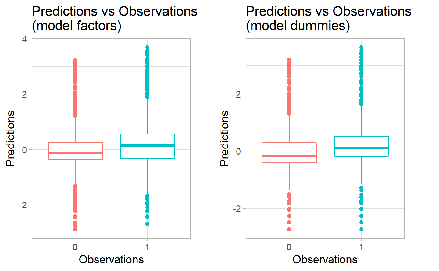
Here we can see some differences in the predictions of the positive category having less variation in the second model. The median of the first model seems to be slightly higher, however the distance between the 1st and 3rd quantiles for the negative category for the second model is a bit higher. It seems that the first model is better at predicting 0 values, while the second is better at predicting positive values. Since our scope is indeed to predict the postive values for the injuries to happen, we could opt for the second one, given the predicitons compared to the test set.