General Analysis
We will start our collision exploration by looking at the boxplot distributions of accidents by month, quarter, weekday, and finally the hour. Moreover, you will find the total number of accidents by weekday (here is the description of the data).
They each have their affiliated comments and interpretations in their tabset sections. Also, please do note that, for simplicity and clarity, our day of the week on the graph starts from Friday.
Boxplot: Monthly Accidents
#> `summarise()` regrouping output by 'date' (override with `.groups` argument)
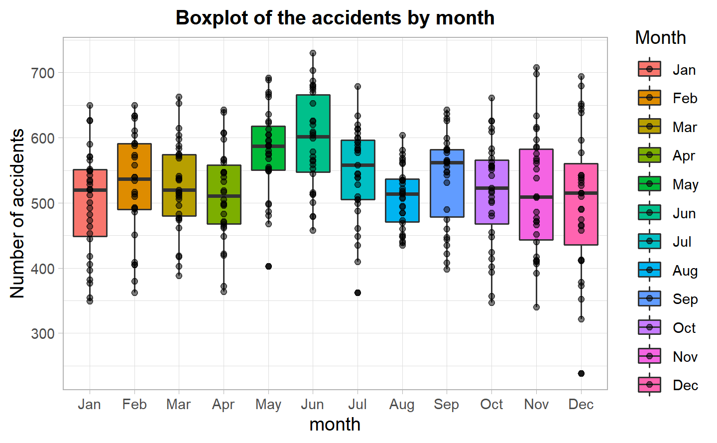
In the first plot, we do see that the accidents as summer approeaches go up, particularly in June, we have the highest number of accidents as well as the highest variation in the number of accidents. The lowest median and variation is in August, which makes sense, as a lot of working people have their annual holidays and probably many people either travel outside the city or stay at home and do not commute as much. There is one date which has particularly low accidents in December, namely the 25th, hence Christmas, as many people celebrate it with their families. In terms of weekdays, it falls on a Wednesday explaining why we have such a low point for that day of the week.
Boxplot: Quarterly
#> `summarise()` regrouping output by 'date' (override with `.groups` argument)
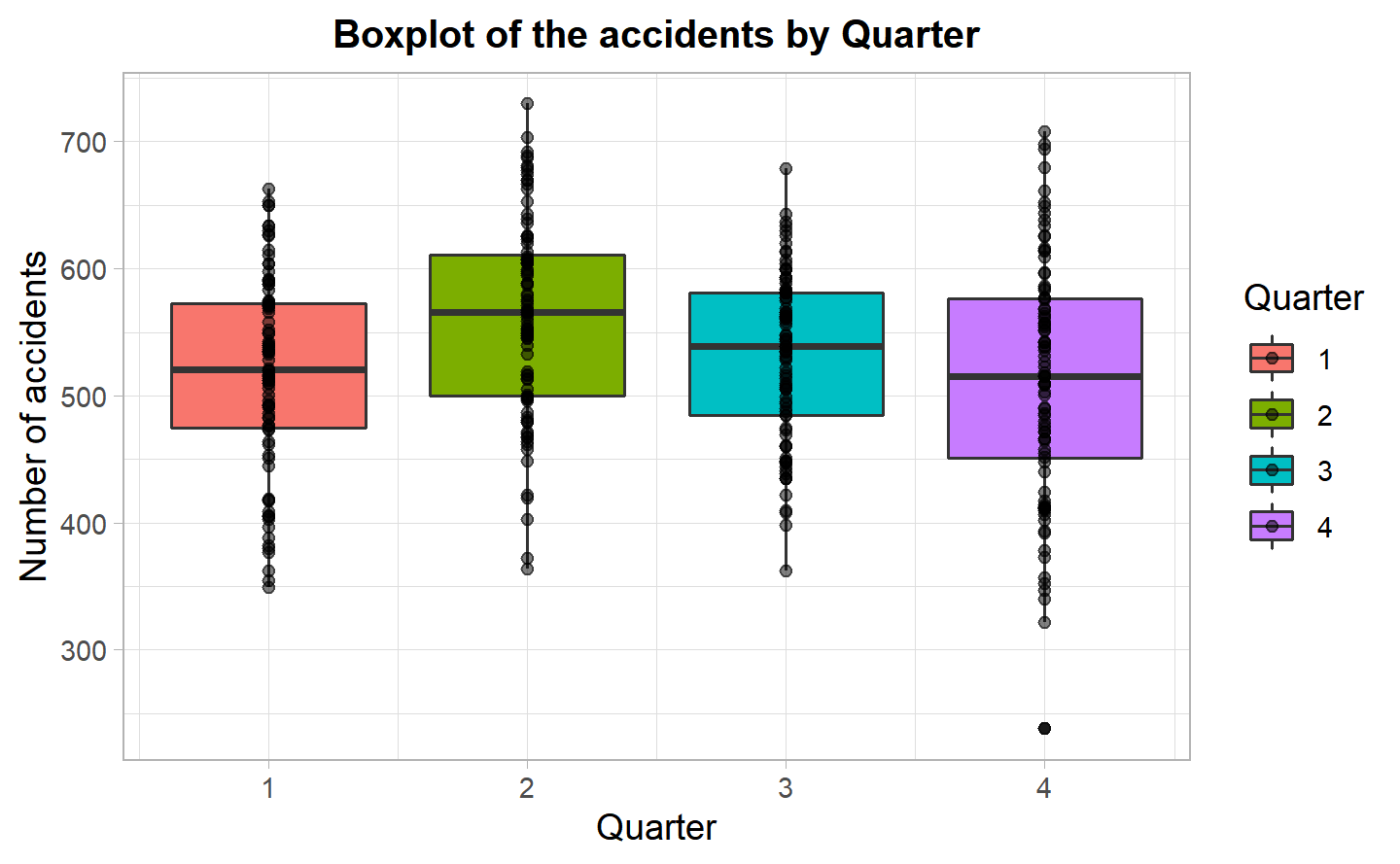
In line with the first plot, the second plot, which shows the distribution of the accidents by quarter, tells us that the second quarter has had the highest number of observed accidents and we can see a decreasing trend from second quarter onwards. The variation seems to be the same among the 1st and 3rd quarter and then somewhat similar between the 2nd and 4th quarter, and we see that in the fourth quarter, which corresponds to fall, the total number of accidents have had the highest variation.
Boxplot: DayMonth
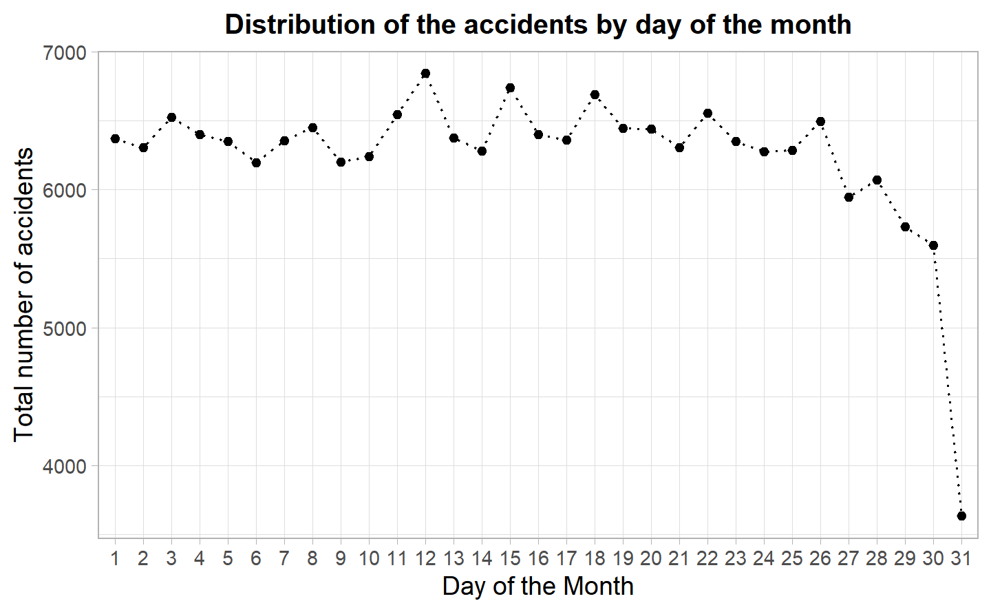
The third plot shows the total number of accidents by day of the month, generally, we can see that in the 12th day of the month as well as in the 14th and 17th we have peaks in accidents. This may not be extremely relevant if we consider what day of the week they correspond to, i.e. 14th could have been a weekday or a weekend during different months, nevertheless, it is interesting to see that there seems to be a peak every 3-4 days from 11th until the 26th.
Boxplot: Weekday
#> `summarise()` regrouping output by 'date' (override with `.groups` argument)

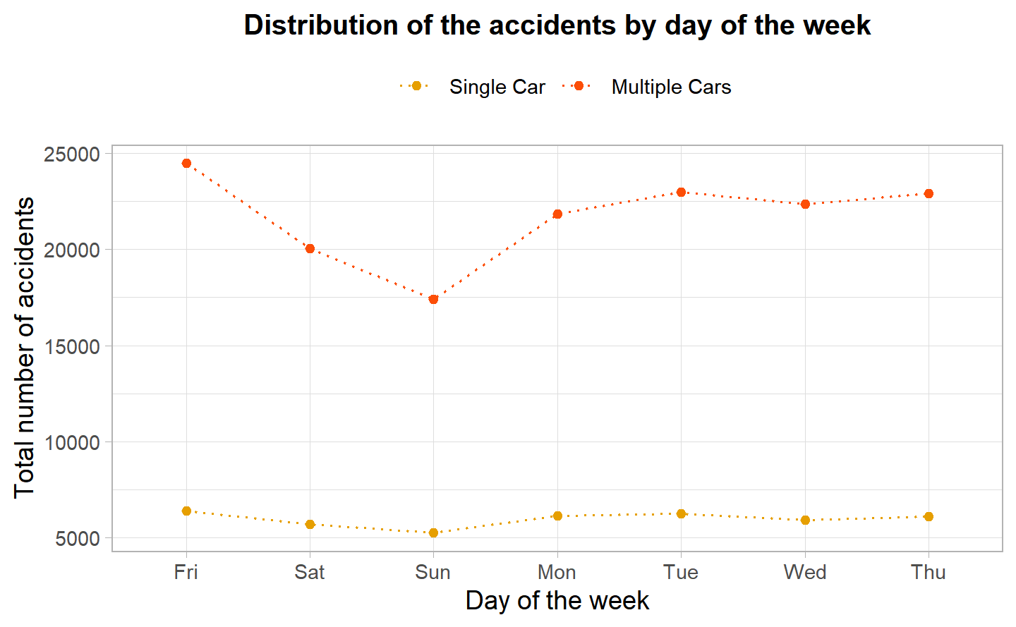
The fourth plot showcases the accident by day of the week, in which we can see that most of the accidents happen on Friday and then this number drastically drops on Saturday to eventually reach its lowest on Sunday. Hence, the weekend seems to play a part in the total number of accidents. This is probably due to fewer people commuting over the weekends, as they may tend to stay inside, hence the rush on Fridays to get home, right before Saturday, increases the total number of accidents. Another possible explanation is that more people are away during the weekend hence explaining the lower number of accidents.
Barplot: Weekday
#> `summarise()` ungrouping output (override with `.groups` argument)
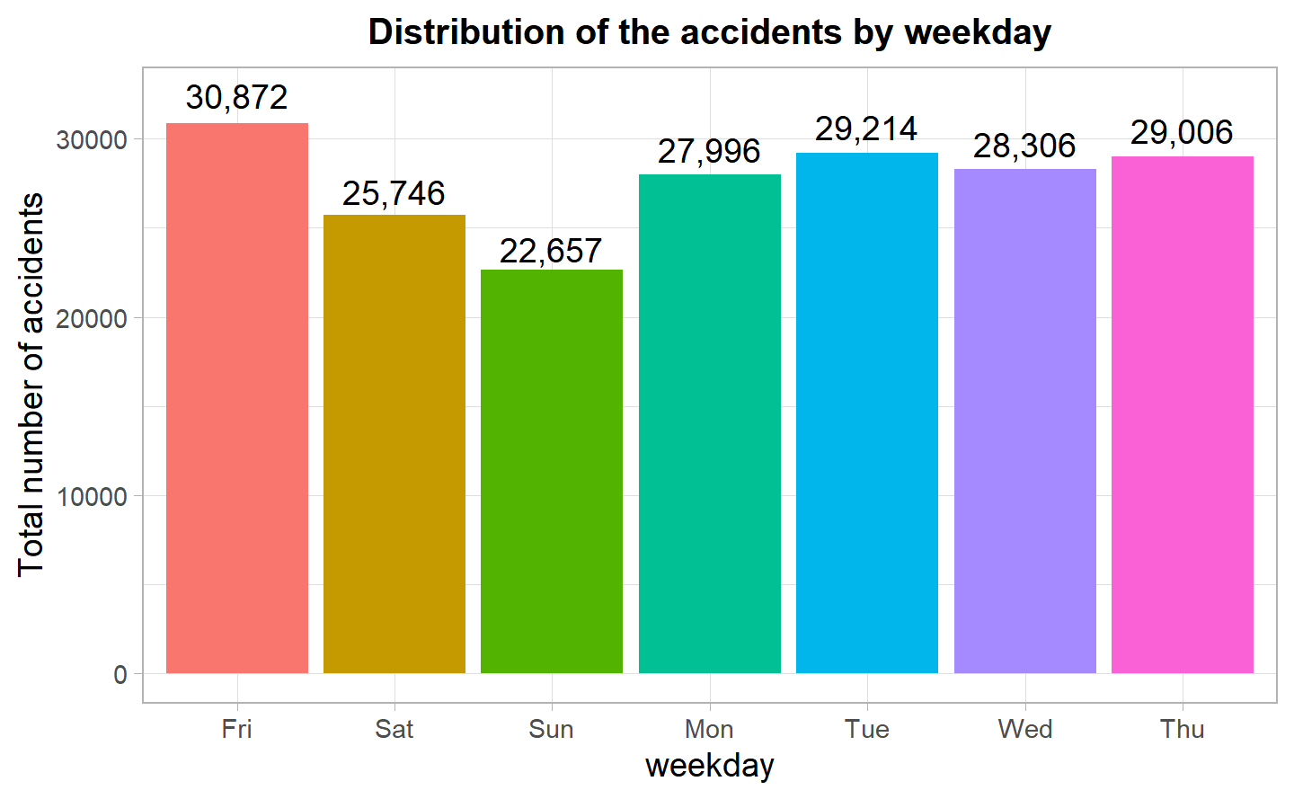
The interpretation of this plot is close to the last one in which, instead of the distribution of accident points, we see the total count. We can still observe that Saturday and Sunday have significantly lower values, while Friday has the highest number of total accidents.
It would be interesting to look at the number of accidents by the hour during the weekend and the weekday to see if there are any clear trends.
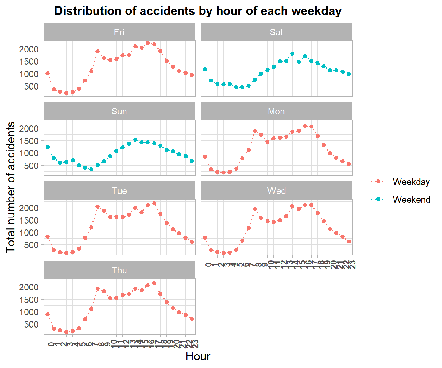
During the weekdays, we can see that from 8:00 to 17:00 we have the most accidents and the diminish going towards the evening. Particularly on Fridays, this number is higher, as there are the two usual peaks at 14:00 and 16:00. The pattern over the weekend fluctuates and only has one peak around 14:00 for both Saturday and Sundays. On Saturdays there is also one at 16:00, which is explainable as, unlike Sundays, on Saturdays many public places and shops are still open.
Single Vs Multiple Cars
Furthermore, we can look at the plots of single vs multiple car accidents considering the time dimension to dive even deeper.
MultipleCars: DayMonth

In the day of the month plot, we can see that the single-car accidents seem to be fairly stable throughout the month, however, multiple cars have many fluctuations, which could indicate that there may be a variable, such as circulation rules or simply the traffic, that is causing more multiple cars accidents than accidents involving cars having a standalone collision with the road objects or pedestrians.
MultipleCars: WeekDay
Furthermore, in the above plot, showing accidents by the weekday, we can see that both types of accidents (i.e.: single and multiple cars) demonstrate similar trends, and, additionally, multiple car accidents seem to fall greatly during Saturday and Sundays, which is in line with our previous hypothesis of people commuting less, hence having less cars on the streets.
MultipleCars: Hour
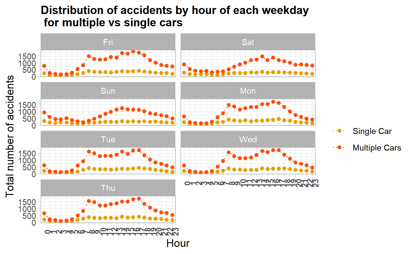
Combining what we have seen from the day of the week, the hour, as well as the single vs multiple car accidents, we can see that in thee plot above, over the weekend, both types of accidents are clearly less volatile and have a reasonable curvature. Additionally, the accidents during different days of the weeks are fairly similar to one another.
### {-}
Relative Injury
Next, we can look at the average probability of injury both per month/day relative to all the accidents in that month/day.
Relative Injury: Monthly
#> `summarise()` ungrouping output (override with `.groups` argument)
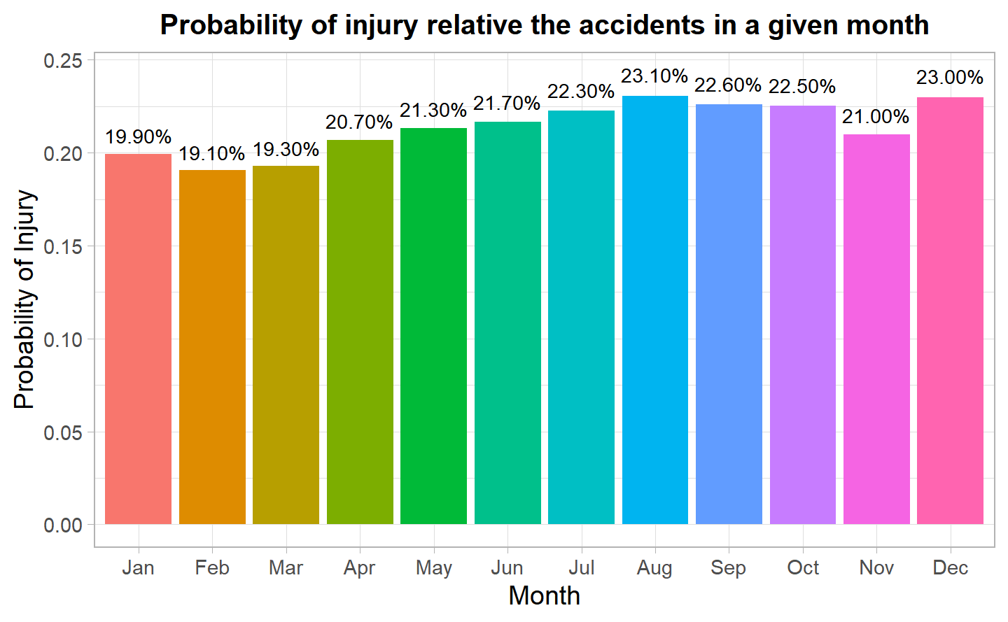
According to the first plot, the highest probability of injuries are in August followed by December. What is interesting to note here, is that there is an increasing trend toward the summer, with a peak in August and a decreasing trend towards December. So that we appear to have a cycle with highest values once during the summer and once during the winter.
Relative Injury: WeekDay
#> `summarise()` ungrouping output (override with `.groups` argument)
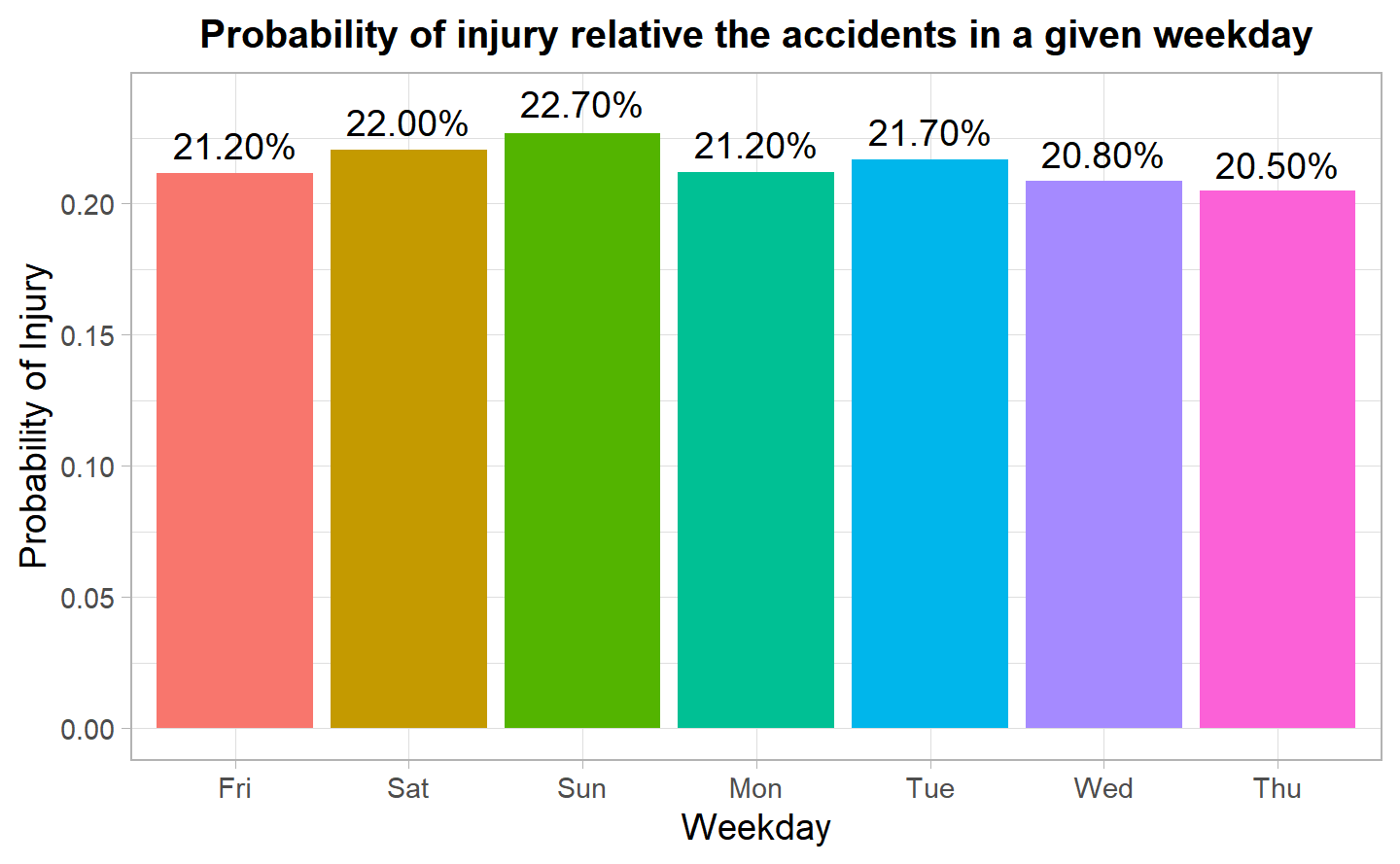
On the other hand, the second plot demonstrates the mean probability of injury in a given day of the week (adjusted for the total number of the accidents). It is extremely interesting to see that, although we initially see the most accidents happen during the week, especially on Fridays, the injuries adjusted for the number of accidents show us that the
probability of an injury during the weekend is the highest. Additionally, during the week most injuries happen on Tuesdays followed by Monday and Thursdays.
Next, we can combine everything we have done to look at four variables of relative injury, weekday, hour and single vs multiple cars at once.
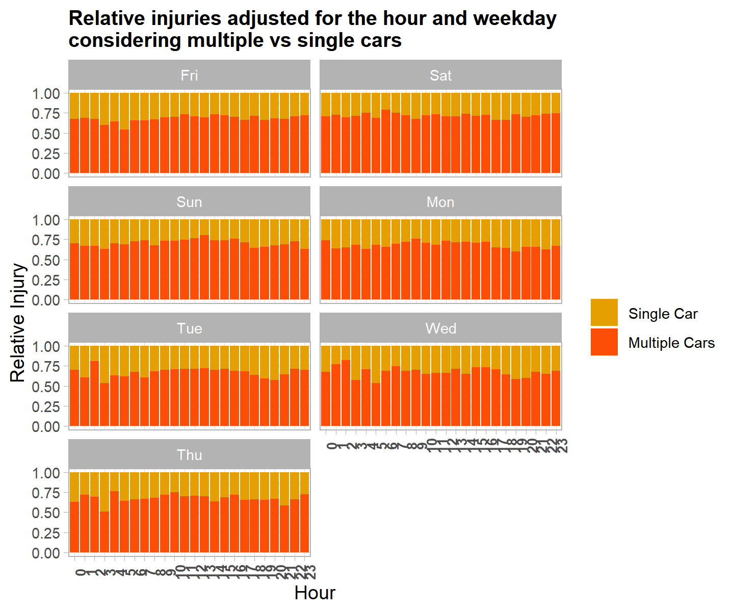
We can see here that even when the probability of injury is adjusted for the time of the accident (the hour and weekday), there are still more multiple car injuries and we rarely have single cars reaching down to 0.5 probability given any day of the week. It is clear that multiple cars have a higher chance of causing an injury, while the probability is less for single cars. This is probably due to the fact that, with more cars involved, there are also more people involved in an accident. Furthermore, we can see that the probability is highest for single-car accidents taking place at 4:00 on a Tuesdays and Thursdays, followed by 5:00 am on Friday and Wednesdays (also 3:00 am on Wednesday seems quite high) and, although this may be surprising at first, it can make sense, as there may not be many people on the street at that hour, hence more accidents that involve a single car take place as the driver is sleepy or not paying full attention. At the same time, it is dark, hence the pedestrian or biker may not be able to see the incoming car. However, the logic of lower traffic density causing less multiple and more single-car injuries may be defied, as accidents do happen at 20:00 and 21:00 on Tuesdays and Wednesdays and although it may not fall within the normal rush hours (8:00 am to 17:00) why particularly that time of the night may be dangerous for a car owner.
Relative Death
Now let’s see the same plots for the probability of having a fatal accident. Both graphs will be interpreted at once right below.
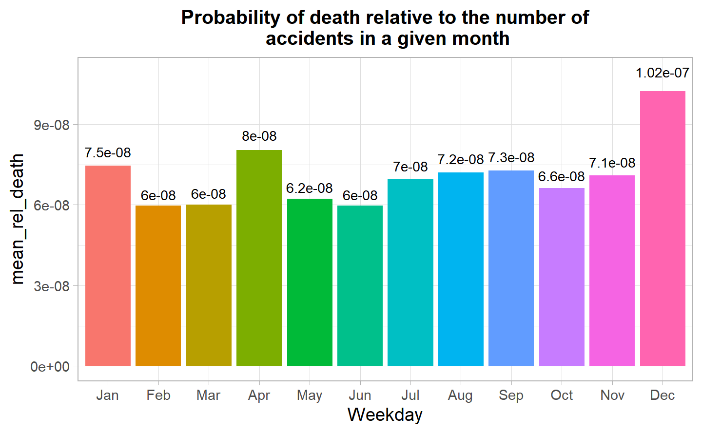
Relative death: Monthly
#> `summarise()` ungrouping output (override with `.groups` argument)
Relative death: WeekDay
#> `summarise()` ungrouping output (override with `.groups` argument)
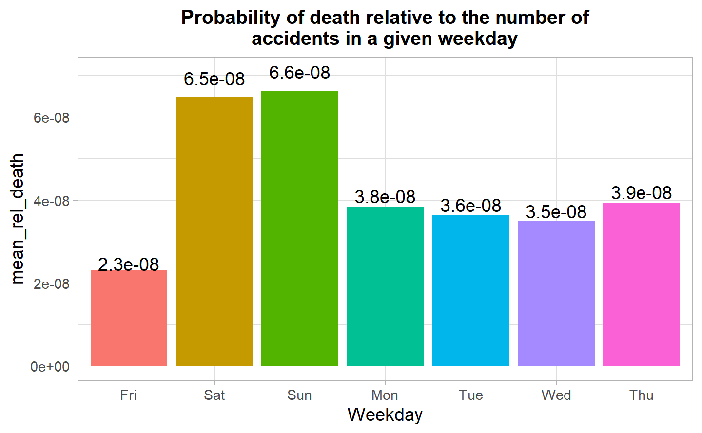
Unlike the injuries, we don’t see the same trend although December seems to be the deadliest month followed by April and January. There is a drastic difference between the months. Moreover, looking at the second plot, there seems to be the most deaths on Saturdays and Sundays, despite the total number of accidents being the lowest during the weekend, this may have to do with drunk driving over the weekend, or other reasons for which people may be a less attentive and aware while driving.
Conclusion of this eda: We will use the weekend as well as the month December as two variables in answering our first research question about the probability of death later in the modelling chapter.
Holiday Analysis
It would be interesting to have a look at the holidays vs normal to say to see how the total number of accidents have evolved as well as the relative chance of injury has evolved.
Table 6.1: NYSE Holidays in 2019
|
Holiday
|
Date
|
Weekday
|
|
New Year’s Day
|
2019-01-01
|
Tue
|
|
Martin Luther King, Jr. Day
|
2019-01-21
|
Mon
|
|
Washington’s Birthday
|
2019-02-18
|
Mon
|
|
Good Friday
|
2019-04-19
|
Fri
|
|
Memorial Day
|
2019-05-27
|
Mon
|
|
Independence Day
|
2019-07-04
|
Thu
|
|
Labor Day
|
2019-09-02
|
Mon
|
|
Thanksgiving Day
|
2019-11-28
|
Thu
|
|
Christmas Day
|
2019-12-25
|
Wed
|
In 2019, there were a total of
9 dates in which there were official holidays in the financial calendar, in which
3398 accidents happened in those particular days.
Now in plotting our variables, we can look at a plot the mean probability of injury in those dates vs any other normal day.
As this may not be a fair comparison due to having too few holidays, we need to also consider the error margins and variations of the same week day. Moreover, we need take into account that if there are more days in a month where it was holidays.
#> `summarise()` regrouping output by 'month' (override with `.groups` argument)
#> `summarise()` ungrouping output (override with `.groups` argument)
#> `summarise()` regrouping output by 'month' (override with `.groups` argument)
#> `summarise()` ungrouping output (override with `.groups` argument)
#> `summarise()` regrouping output by 'month' (override with `.groups` argument)

Table 6.2: Probability of injury during holidays arranged by the day of the week
|
Holiday
|
Date
|
Weekday
|
Month
|
mean_injured
|
|
Good Friday
|
2019-04-19
|
Fri
|
Apr
|
0.233
|
|
Martin Luther King, Jr. Day
|
2019-01-21
|
Mon
|
Jan
|
0.207
|
|
Washington’s Birthday
|
2019-02-18
|
Mon
|
Feb
|
0.184
|
|
Memorial Day
|
2019-05-27
|
Mon
|
May
|
0.295
|
|
Labor Day
|
2019-09-02
|
Mon
|
Sep
|
0.211
|
|
Independence Day
|
2019-07-04
|
Thu
|
Jul
|
0.265
|
|
Thanksgiving Day
|
2019-11-28
|
Thu
|
Nov
|
0.188
|
|
New Year’s Day
|
2019-01-01
|
Tue
|
Jan
|
0.252
|
|
Christmas Day
|
2019-12-25
|
Wed
|
Dec
|
0.202
|
There are only two holidays that fell on a Friday and a Wednesday and they appear to be outside the range of probability of injury in those days. While the first is the Good Friday on April the 19th, the second one is the New Year’s Day which was on a Tuesday in 2019, explaining why it values is much higher than the usual.
The day with the most probability of injury is Memorial day on Monday the 27th, while the second-highest day is July the 4th on a Thursday, also known as the Independence Day.
Visually, it appears that some holidays exceed the range, which is interesting itself if you consider the type of the holidays in the culture, such as New Year’s Eve or July the 4th, that emphasis going out, compared to other holidays, such as Washington’s Birthday, which is perhaps a less known holiday for outdoor celebrations. Also, Thanksgiving day emphasis on staying with the family and we can see that, as fewer people may be travelling constantly on the road (they still have to travel to a friend’s/family’s place to dine), we still have a normal probability of injuries compared to any other Thursday in the year.
Source of NYSE holidays.