4 Weather EDA
4.1 Variable organization
In this section we will import our cleaned data and rename some of the variables for clarity and simplicity. Then, we will start our analysis by the exploration of the weather data (here is the description of the data).
Firstly, we write a function to make all the variable names in our dataset coherent and replace the space between the words with a "_", which will make it easier for us to use them in the code. Furthermore, if they are longer than 3 words, we remove the rest of the words.
Then, we create two datasets (accidents_numerical and accidents_simplified) which we will use throughout our analysis for different purposes. The difference between them is that one (accidents_numerical) only contains contributing factors, which we will use in the variable selection chapter, while the other (accidents simplified) does not contain any of the contributing factors, which, as the name suggests, makes it simpler to use, and will be extensively employed in this chapter.
4.2 Weather exploration
4.2.1 Creating categories and weather definitions
We would like to create a factor variable divided in light, moderate and heavy for the rain, snow and the wind variables. Moreover, we want to find a way to use only one of the two variables that is considering snow (ie: snow and snwd).
#> `summarise()` regrouping output by 'date', 'awnd', 'snow', 'prcp' (override with `.groups` argument)This graph is pretty informative. We can see that the snow variable is positive only on a few days, all situated in 4 months (January, February, March and December), as one could have imagined. Moreover, we can see that the wind has no information for the two first months, but from the second week of March becomes the most important variable, with the highest variation and the highest presence throughout the year. We can also see that there is an increase towards the end of the year. The rainfall variable seems to be quite related to both the snowfall and the wind variables. We can see that it takes small values, meaning that when it rains (and it seems not to have happened often in NYC in 2019), it is quite light as rainfall.
Before diving deeper, we will create 3 functions that would help to avoid repetition: (1) that will give us the number of times an accident has happened at different levels of that weather, (2) one showing us the correlation of that particular weather metric with the other variables and (3) one to summarize the distribution of that weather metric.
Let’s move on with the weather analysis starting with the snow variable.
4.2.1.1 Snowfall (snow)
The snow variable measures and records the snowfall (snow, ice pellets) since the previous snowfall observation (24 hours) per day thorughout the year (source). Hence, if the snowfall is equal to 0 it means that it hasn’t snowed, while, if it takes positive values, we can see how heavily it has been snowing.
As already mentioned, from the previous graph (??), we can see that the month with the highest value of snowfall is March, and that, as one could expect, the data from April to November are equal to zero. Moreover, we can see that throughout the year it snowed only 14 times, all of them are limited to the months of January, February, March and December.
4.2.1.1.1 Levels of Snowfall & number of accidents
| snow | n_accidents |
|---|---|
| 0.0 | 185,978 |
| 1.3 | 1,109 |
| 0.2 | 972 |
| 1.4 | 653 |
| 0.7 | 644 |
| 0.1 | 634 |
| 1.2 | 634 |
| 4.0 | 604 |
| 0.3 | 577 |
| 0.5 | 552 |
| 0.4 | 501 |
| 3.0 | 477 |
| 2.0 | 462 |
4.2.1.1.2 Summary Statistics of Snowfall
| summary Metric | value |
|---|---|
| Min. | 0.10 |
| 1st Qu. | 0.30 |
| Median | 1.20 |
| Mean | 1.18 |
| 3rd Qu. | 1.40 |
| Max. | 4.00 |
4.2.1.1.3 Correlation of Snowfall and other variables
| other_variables | snow |
|---|---|
| snwd | 0.72 |
| wt01 | 0.17 |
| day | -0.15 |
| monthday | -0.15 |
| awnd | -0.14 |
| prcp | 0.12 |
| multiple_cars | -0.02 |
| latitude | -0.01 |
| longitude | -0.01 |
| persons_injured | -0.01 |
| pedestrians_injured | 0.01 |
| cyclist_injured | -0.01 |
| motorist_injured | -0.01 |
| hour | -0.01 |
| persons_killed | 0.00 |
| pedestrians_killed | 0.00 |
| cyclist_killed | 0.00 |
| motorist_killed | 0.00 |
| postvz_sl | 0.00 |
Regarding the correlation, the highest ones for snow are found with the variables snwd, wt01, day (negatively), awnd (negatively) and prcp.
#> `summarise()` regrouping output by 'snow_fac' (override with `.groups` argument)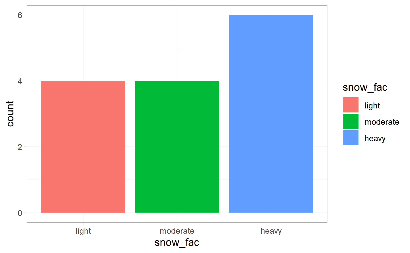
We have created the level of the factor variable for snow based on its quantiles. Of course, the majority of the days have no snow, but of the 14 the days that had had snow, we had 6 having “heavy” amount of snow (based on our factor level), and 4 with respectively a “light” and a “moderate” amount.
4.2.1.2 Snow depth (snwd)
Now let’s have a look at the snwd variable, which we are expecting to be highly correlated to the snow variable. Once again, the unit of the values is in inches, and it determines the depth of the new and old snow remaining on the ground that there were in NYC in a given day (source). Hence, it goes the same as for the snow variable: if the value is zero it means that there has not been snow on the streets, while if it positive, it gives how much of it there was.
#> `summarise()` regrouping output by 'date' (override with `.groups` argument)| date | snwd |
|---|---|
| 2019-01-18 | 1.2 |
| 2019-02-13 | 1.2 |
| 2019-02-21 | 1.2 |
| 2019-03-01 | 1.2 |
| 2019-03-02 | 3.9 |
| 2019-03-03 | 1.2 |
| 2019-03-04 | 3.9 |
| 2019-03-05 | 2.0 |
| 2019-03-06 | 1.2 |
| 2019-03-07 | 1.2 |
| 2019-12-03 | 1.2 |
#> `summarise()` regrouping output by 'date' (override with `.groups` argument)
#> `summarise()` ungrouping output (override with `.groups` argument)
As we can see, regarding snow depth, there are only 4 different levels (ie.: 0, 1.2, 3.9, 2), and the value was positive only for 11 days in the year (ie 2019-01-18, 2019-02-13, 2019-02-21, 2019-03-01, 2019-03-02, 2019-03-03, 2019-03-04, 2019-03-05, 2019-03-06, 2019-03-07, 2019-12-03). “Heavy” snow generally means snowfall accumulating to 6" or more in depth in 24 hours or less (https://forecast.weather.gov/glossary.php?word=heavy%20snow), as we can see here the maximum value it has taken in 2019 has been 3.9 inches. Hence, we have decided to determine the values of the factorial variable based on the distribution of the data we have, as you can see just below.
4.2.1.2.1 Levels of Snow Depth & number of accidents
| snwd | n_accidents |
|---|---|
| 0.0 | 187,707 |
| 1.2 | 4,441 |
| 3.9 | 1,066 |
| 2.0 | 583 |
4.2.1.2.2 Summary Statistics of Snow Depth
| summary Metric | value |
|---|---|
| Min. | 1.20 |
| 1st Qu. | 1.20 |
| Median | 1.20 |
| Mean | 1.75 |
| 3rd Qu. | 2.00 |
| Max. | 3.90 |
4.2.1.2.3 Correlation of Snow Depth and other variables
| other_variables | snwd |
|---|---|
| snow | 0.72 |
| awnd | -0.19 |
| day | -0.17 |
| monthday | -0.17 |
| wt01 | 0.10 |
| prcp | 0.03 |
| hour | -0.02 |
| longitude | -0.01 |
| persons_injured | -0.01 |
| cyclist_injured | -0.01 |
| motorist_injured | -0.01 |
| multiple_cars | -0.01 |
| latitude | 0.00 |
| persons_killed | 0.00 |
| pedestrians_injured | 0.00 |
| pedestrians_killed | 0.00 |
| cyclist_killed | 0.00 |
| motorist_killed | 0.00 |
| postvz_sl | 0.00 |
The variables with the highest correlation with snwd are snow, awnd (negatively), day (negatively), and wt01. This is quite predictable by the definition of wt01, and by the fact that, if there is snow depth, it probably snowed the same day or the day before, moreover it is quite normal to have wind when it is snowing.
#> `summarise()` regrouping output by 'snwd_fac' (override with `.groups` argument)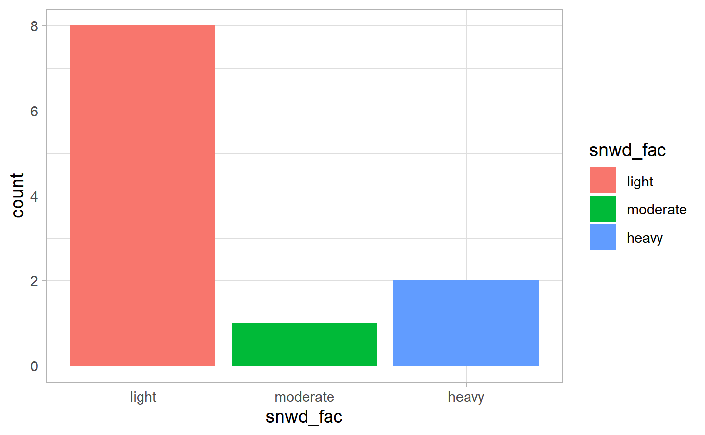
We used the quantile of the variables (without considering the observations = 0) to create the level for the factor variables. Of course, the majority of days had no snow width, as one could have imagined. However, when it had had snow, the amount of depth is “light” in the majority of cases.
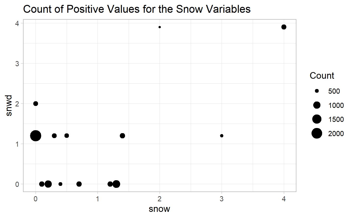
The times in which snow is positive and snwd is null are probably due to the fact that the snow melted before it was possible to measure it. On the other hand, a positive depth without snowfall could mean that the snow remained for more days than it snowed (because it froze, for example). In general we can see that the two variables seem to be positively correlated.
#> `summarise()` regrouping output by 'snow_fac', 'snwd_fac' (override with `.groups` argument)| snow_fac | snwd_fac | date | count |
|---|---|---|---|
| light | light | 2019-12-03 | 577 |
| heavy | heavy | 2019-03-02 | 604 |
| heavy | heavy | 2019-03-04 | 462 |
#> `summarise()` regrouping output by 'snow_fac' (override with `.groups` argument)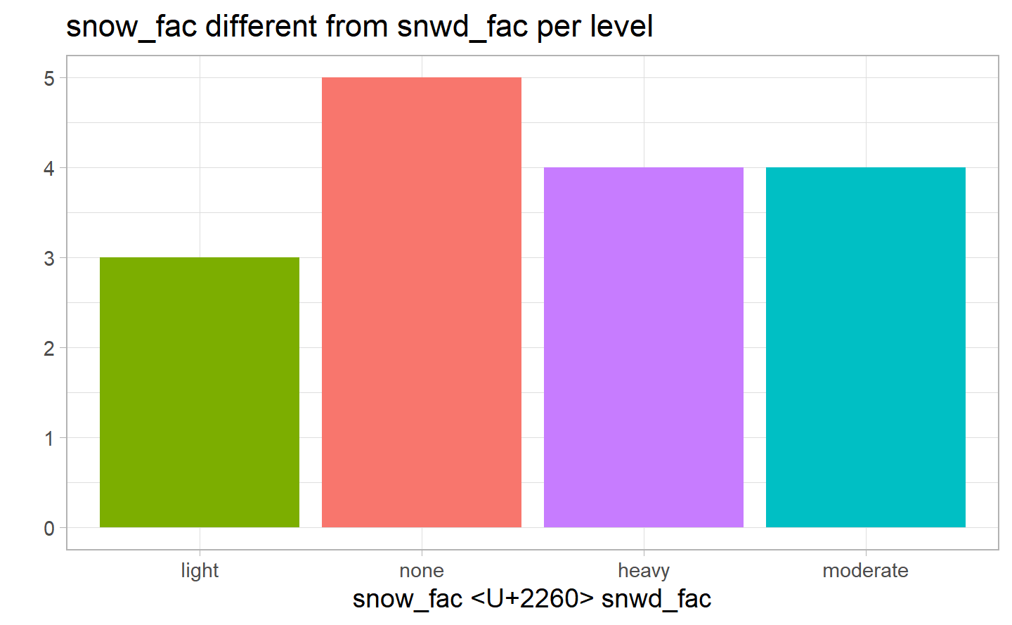
This plot shows the difference between the two factorial variables for snow that we have just created having different values. Of course, the vast majority of instances in which the two variables take the same level is when both are equal to “none”, which is not really informative. However, as we can see from the table above, the only days in which they are equal and different from “none” is the 03-02-2019 and 04-03-2019 being both “heavy” and the 03-12-2019 being both “light”. While, from the graph above, the days in which the two variables take different values, are mainly due to when snow_fac has level “none”. All these values are quite low, because the snowfall was positive only for a dozen of days in NYC in 2019.
4.2.1.3 Average wind speed (awnd)
Now let’s look at the variable awnd, which is the variable considering the speed of the wind in mph per day. If the value is equal to zero, it means there has been no wind on that day, while, if it positive, it gives the average speed of the wind. We have already seen in figure ??, the first two months of the year have missing values, and there is an increase towards the end of the year.
#> `stat_bin()` using `bins = 30`. Pick better value with `binwidth`.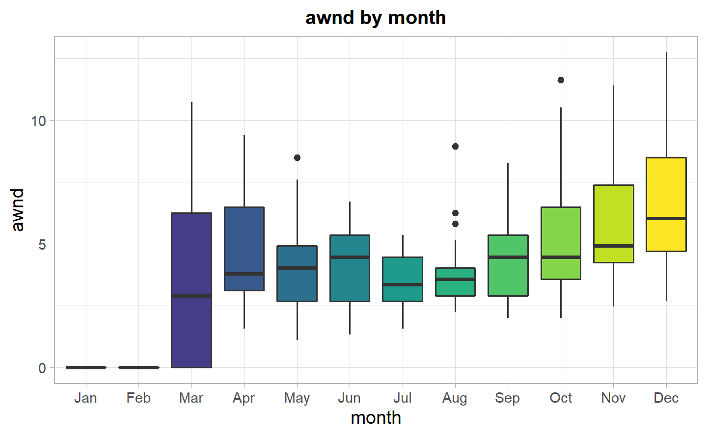
The boxplot confirms the fact that there is an increase of the speed of wind towards the end of the year. In general, this variable has a majority of zero values. If positive, though, we can see that the peak is around 4mph. There could be a problem, as it seems to be a zero-inflated variable. But, once again, this zero inflated data is given by the fact that there are no observations for the first two months.
This time we will do the things differently and look at the wind by dates.
#> `summarise()` regrouping output by 'date' (override with `.groups` argument)| date | awnd |
|---|---|
| 2019-03-11 | 9.17 |
| 2019-03-12 | 8.95 |
| 2019-03-13 | 2.46 |
| 2019-03-14 | 2.91 |
| 2019-03-15 | 2.24 |
| 2019-03-16 | 10.07 |
| 2019-03-17 | 6.26 |
| 2019-03-18 | 2.01 |
| 2019-03-19 | 3.13 |
| 2019-03-20 | 2.91 |
| 2019-03-21 | 7.83 |
| 2019-03-22 | 10.74 |
| 2019-03-23 | 9.84 |
| 2019-03-24 | 4.47 |
| 2019-03-25 | 4.25 |
| 2019-03-26 | 7.83 |
| 2019-03-27 | 4.03 |
| 2019-03-28 | 1.57 |
| 2019-03-29 | 2.01 |
| 2019-03-30 | 3.36 |
| 2019-03-31 | 5.82 |
| 2019-04-01 | 7.16 |
| 2019-04-02 | 4.47 |
| 2019-04-03 | 7.38 |
| 2019-04-04 | 6.71 |
| 2019-04-05 | 5.82 |
| 2019-04-06 | 3.36 |
| 2019-04-07 | 1.57 |
| 2019-04-08 | 3.58 |
| 2019-04-09 | 2.91 |
| 2019-04-10 | 6.49 |
| 2019-04-11 | 3.13 |
| 2019-04-12 | 3.80 |
| 2019-04-13 | 2.91 |
| 2019-04-14 | 1.57 |
| 2019-04-15 | 8.50 |
| 2019-04-16 | 9.40 |
| 2019-04-17 | 3.13 |
| 2019-04-18 | 3.58 |
| 2019-04-19 | 3.36 |
| 2019-04-20 | 3.80 |
| 2019-04-21 | 3.36 |
| 2019-04-22 | 4.47 |
| 2019-04-23 | 2.01 |
| 2019-04-24 | 5.82 |
| 2019-04-25 | 3.36 |
| 2019-04-26 | 4.92 |
| 2019-04-27 | 6.93 |
| 2019-04-28 | 3.80 |
| 2019-04-29 | 2.68 |
| 2019-04-30 | 2.01 |
| 2019-05-01 | 2.46 |
| 2019-05-02 | 2.68 |
| 2019-05-03 | 2.46 |
| 2019-05-04 | 1.12 |
| 2019-05-05 | 7.16 |
| 2019-05-06 | 4.03 |
| 2019-05-07 | 1.34 |
| 2019-05-08 | 4.47 |
| 2019-05-09 | 5.59 |
| 2019-05-10 | 1.57 |
| 2019-05-11 | 3.13 |
| 2019-05-12 | 8.50 |
| 2019-05-13 | 5.59 |
| 2019-05-14 | 2.24 |
| 2019-05-15 | 3.80 |
| 2019-05-16 | 2.68 |
| 2019-05-17 | 4.92 |
| 2019-05-18 | 2.68 |
| 2019-05-19 | 2.91 |
| 2019-05-20 | 5.37 |
| 2019-05-21 | 5.82 |
| 2019-05-22 | 4.25 |
| 2019-05-23 | 4.03 |
| 2019-05-24 | 7.61 |
| 2019-05-25 | 4.03 |
| 2019-05-26 | 4.25 |
| 2019-05-27 | 3.58 |
| 2019-05-28 | 4.25 |
| 2019-05-29 | 4.70 |
| 2019-05-30 | 2.01 |
| 2019-05-31 | 2.68 |
| 2019-06-01 | 2.68 |
| 2019-06-02 | 3.80 |
| 2019-06-03 | 5.37 |
| 2019-06-04 | 3.80 |
| 2019-06-05 | 4.47 |
| 2019-06-06 | 4.70 |
| 2019-06-07 | 2.24 |
| 2019-06-08 | 6.26 |
| 2019-06-09 | 6.49 |
| 2019-06-10 | 6.71 |
| 2019-06-11 | 6.26 |
| 2019-06-12 | 4.03 |
| 2019-06-13 | 5.82 |
| 2019-06-14 | 6.04 |
| 2019-06-15 | 4.47 |
| 2019-06-16 | 5.14 |
| 2019-06-17 | 1.34 |
| 2019-06-18 | 1.79 |
| 2019-06-19 | 2.91 |
| 2019-06-20 | 3.13 |
| 2019-06-21 | 5.14 |
| 2019-06-22 | 5.59 |
| 2019-06-23 | 4.70 |
| 2019-06-24 | 1.79 |
| 2019-06-25 | 2.01 |
| 2019-06-26 | 3.13 |
| 2019-06-27 | 2.68 |
| 2019-06-28 | 2.46 |
| 2019-06-29 | 4.70 |
| 2019-06-30 | 5.14 |
| 2019-07-01 | 4.47 |
| 2019-07-02 | 2.46 |
| 2019-07-03 | 1.79 |
| 2019-07-04 | 2.68 |
| 2019-07-05 | 2.91 |
| 2019-07-06 | 3.36 |
| 2019-07-07 | 4.92 |
| 2019-07-08 | 2.68 |
| 2019-07-09 | 2.68 |
| 2019-07-10 | 2.46 |
| 2019-07-11 | 4.47 |
| 2019-07-12 | 5.14 |
| 2019-07-13 | 3.80 |
| 2019-07-14 | 4.92 |
| 2019-07-15 | 2.91 |
| 2019-07-16 | 2.91 |
| 2019-07-17 | 3.58 |
| 2019-07-18 | 4.92 |
| 2019-07-19 | 3.58 |
| 2019-07-20 | 4.25 |
| 2019-07-21 | 4.47 |
| 2019-07-22 | 2.68 |
| 2019-07-23 | 4.03 |
| 2019-07-24 | 2.91 |
| 2019-07-25 | 1.79 |
| 2019-07-26 | 1.57 |
| 2019-07-27 | 2.91 |
| 2019-07-28 | 5.37 |
| 2019-07-29 | 4.47 |
| 2019-07-30 | 3.36 |
| 2019-07-31 | 2.91 |
| 2019-08-01 | 2.24 |
| 2019-08-02 | 3.58 |
| 2019-08-03 | 3.58 |
| 2019-08-04 | 2.68 |
| 2019-08-05 | 4.47 |
| 2019-08-06 | 3.13 |
| 2019-08-07 | 2.68 |
| 2019-08-08 | 4.70 |
| 2019-08-09 | 3.58 |
| 2019-08-10 | 5.14 |
| 2019-08-11 | 3.13 |
| 2019-08-12 | 3.58 |
| 2019-08-13 | 3.58 |
| 2019-08-14 | 3.58 |
| 2019-08-15 | 4.03 |
| 2019-08-16 | 2.68 |
| 2019-08-17 | 3.36 |
| 2019-08-18 | 2.24 |
| 2019-08-19 | 2.91 |
| 2019-08-20 | 2.91 |
| 2019-08-21 | 2.91 |
| 2019-08-22 | 3.80 |
| 2019-08-23 | 3.36 |
| 2019-08-24 | 5.14 |
| 2019-08-25 | 8.95 |
| 2019-08-26 | 6.26 |
| 2019-08-27 | 3.13 |
| 2019-08-28 | 3.80 |
| 2019-08-29 | 4.03 |
| 2019-08-30 | 4.03 |
| 2019-08-31 | 5.82 |
| 2019-09-01 | 4.47 |
| 2019-09-02 | 2.46 |
| 2019-09-03 | 3.36 |
| 2019-09-04 | 3.80 |
| 2019-09-05 | 5.14 |
| 2019-09-06 | 8.28 |
| 2019-09-07 | 4.47 |
| 2019-09-08 | 2.24 |
| 2019-09-09 | 4.47 |
| 2019-09-10 | 2.91 |
| 2019-09-11 | 5.14 |
| 2019-09-12 | 4.92 |
| 2019-09-13 | 6.49 |
| 2019-09-14 | 2.91 |
| 2019-09-15 | 2.24 |
| 2019-09-16 | 2.01 |
| 2019-09-17 | 5.59 |
| 2019-09-18 | 6.49 |
| 2019-09-19 | 2.91 |
| 2019-09-20 | 4.70 |
| 2019-09-21 | 2.68 |
| 2019-09-22 | 3.58 |
| 2019-09-23 | 5.37 |
| 2019-09-24 | 5.82 |
| 2019-09-25 | 3.36 |
| 2019-09-26 | 3.58 |
| 2019-09-27 | 3.58 |
| 2019-09-28 | 2.91 |
| 2019-09-29 | 6.26 |
| 2019-09-30 | 6.93 |
| 2019-10-01 | 3.80 |
| 2019-10-02 | 6.49 |
| 2019-10-03 | 6.26 |
| 2019-10-04 | 6.93 |
| 2019-10-05 | 4.92 |
| 2019-10-06 | 2.91 |
| 2019-10-07 | 4.03 |
| 2019-10-08 | 7.83 |
| 2019-10-09 | 10.51 |
| 2019-10-10 | 9.62 |
| 2019-10-11 | 9.17 |
| 2019-10-12 | 3.58 |
| 2019-10-13 | 2.01 |
| 2019-10-14 | 4.03 |
| 2019-10-15 | 2.91 |
| 2019-10-16 | 6.49 |
| 2019-10-17 | 11.63 |
| 2019-10-18 | 8.72 |
| 2019-10-19 | 2.68 |
| 2019-10-20 | 4.47 |
| 2019-10-21 | 4.03 |
| 2019-10-22 | 4.47 |
| 2019-10-23 | 6.26 |
| 2019-10-24 | 3.13 |
| 2019-10-25 | 2.91 |
| 2019-10-26 | 3.36 |
| 2019-10-27 | 4.92 |
| 2019-10-28 | 3.58 |
| 2019-10-29 | 4.03 |
| 2019-10-30 | 3.13 |
| 2019-10-31 | 5.14 |
| 2019-11-01 | 9.40 |
| 2019-11-02 | 3.80 |
| 2019-11-03 | 4.92 |
| 2019-11-04 | 3.13 |
| 2019-11-05 | 2.91 |
| 2019-11-06 | 4.92 |
| 2019-11-07 | 4.70 |
| 2019-11-08 | 7.61 |
| 2019-11-09 | 3.13 |
| 2019-11-10 | 3.80 |
| 2019-11-11 | 2.46 |
| 2019-11-12 | 9.40 |
| 2019-11-13 | 5.37 |
| 2019-11-14 | 4.25 |
| 2019-11-15 | 4.25 |
| 2019-11-16 | 10.29 |
| 2019-11-17 | 10.51 |
| 2019-11-18 | 6.04 |
| 2019-11-19 | 4.47 |
| 2019-11-20 | 5.14 |
| 2019-11-21 | 4.47 |
| 2019-11-22 | 7.38 |
| 2019-11-23 | 4.25 |
| 2019-11-24 | 8.05 |
| 2019-11-25 | 5.14 |
| 2019-11-26 | 4.25 |
| 2019-11-27 | 4.25 |
| 2019-11-28 | 11.41 |
| 2019-11-29 | 6.26 |
| 2019-11-30 | 4.25 |
| 2019-12-01 | 9.84 |
| 2019-12-02 | 8.50 |
| 2019-12-03 | 7.16 |
| 2019-12-04 | 5.37 |
| 2019-12-05 | 9.40 |
| 2019-12-06 | 7.38 |
| 2019-12-07 | 6.93 |
| 2019-12-08 | 2.68 |
| 2019-12-09 | 4.47 |
| 2019-12-10 | 6.93 |
| 2019-12-11 | 6.26 |
| 2019-12-12 | 4.70 |
| 2019-12-13 | 5.82 |
| 2019-12-14 | 6.04 |
| 2019-12-15 | 9.62 |
| 2019-12-16 | 3.80 |
| 2019-12-17 | 8.72 |
| 2019-12-18 | 8.95 |
| 2019-12-19 | 10.51 |
| 2019-12-20 | 6.04 |
| 2019-12-21 | 2.91 |
| 2019-12-22 | 4.70 |
| 2019-12-23 | 4.70 |
| 2019-12-24 | 5.82 |
| 2019-12-25 | 3.58 |
| 2019-12-26 | 5.82 |
| 2019-12-27 | 4.47 |
| 2019-12-28 | 4.03 |
| 2019-12-29 | 4.92 |
| 2019-12-30 | 12.75 |
| 2019-12-31 | 5.14 |
#> `summarise()` regrouping output by 'date' (override with `.groups` argument)NYC seems to be a windy place, taking into consideration the fact that we have 69 days of missing data (having the first value the 11 March 2019)! As we have already seen in the first graph of this section (??), the value for the wind was positive for almost everyday, after the first positive observation.
4.2.1.3.1 Levels of Average Wind Speed & number of accidents
| awnd | n_accidents |
|---|---|
| 0.00 | 35,602 |
| 2.91 | 12,567 |
| 4.47 | 10,688 |
| 2.68 | 9,198 |
| 3.58 | 8,702 |
| 4.03 | 7,275 |
| 3.13 | 7,054 |
| 3.80 | 6,958 |
| 5.14 | 6,545 |
| 3.36 | 5,999 |
| 4.25 | 5,839 |
| 4.70 | 5,749 |
| 4.92 | 5,504 |
| 5.82 | 5,356 |
| 6.26 | 4,629 |
| 2.01 | 4,269 |
| 2.46 | 4,219 |
| 2.24 | 3,840 |
| 6.49 | 3,448 |
| 5.37 | 3,355 |
| 1.57 | 2,663 |
| 6.93 | 2,652 |
| 6.04 | 2,544 |
| 1.79 | 2,491 |
| 9.40 | 2,386 |
| 5.59 | 2,280 |
| 8.50 | 1,693 |
| 7.38 | 1,666 |
| 7.83 | 1,626 |
| 8.95 | 1,622 |
| 7.16 | 1,611 |
| 10.51 | 1,403 |
| 7.61 | 1,281 |
| 8.72 | 1,221 |
| 6.71 | 1,166 |
| 9.17 | 1,155 |
| 1.34 | 1,103 |
| 9.62 | 1,028 |
| 9.84 | 856 |
| 10.74 | 663 |
| 11.63 | 554 |
| 8.28 | 543 |
| 10.07 | 506 |
| 1.12 | 499 |
| 12.75 | 491 |
| 10.29 | 486 |
| 8.05 | 472 |
| 11.41 | 340 |
4.2.1.3.2 Summary Statistics of Average Wind Speed
| summary Metric | value |
|---|---|
| Min. | 1.12 |
| 1st Qu. | 2.91 |
| Median | 4.25 |
| Mean | 4.66 |
| 3rd Qu. | 5.82 |
| Max. | 12.75 |
4.2.1.3.3 Correlation of Wind and other variables
| other_variables | awnd |
|---|---|
| snwd | -0.19 |
| snow | -0.14 |
| prcp | 0.11 |
| wt01 | 0.05 |
| longitude | 0.02 |
| persons_injured | 0.02 |
| day | 0.02 |
| monthday | 0.02 |
| latitude | 0.01 |
| pedestrians_injured | 0.01 |
| motorist_injured | 0.01 |
| postvz_sl | 0.01 |
| persons_killed | 0.00 |
| pedestrians_killed | 0.00 |
| cyclist_injured | 0.00 |
| cyclist_killed | 0.00 |
| motorist_killed | 0.00 |
| multiple_cars | 0.00 |
| hour | 0.00 |
There are 48 different values for the average of wind throughout the year. The range is between 0, 12.75 mph. In the first table we can see the number of obsevation for each value of the variable. The second table gives the distribution of the variable and its main quantiles, with the mean at 4.664, the median at 4.25, the 1st and 3rd quantiles respectivels at 2.91 and 5.82. This values have been calulated by not considering the days in which there wasn’t wind (so when the value of awnd = 0). We want to see, if there is wind, what is its value. Finally, the highest correlation are negatively to snwd, snow, and positively prcp, however they are all below 20%.
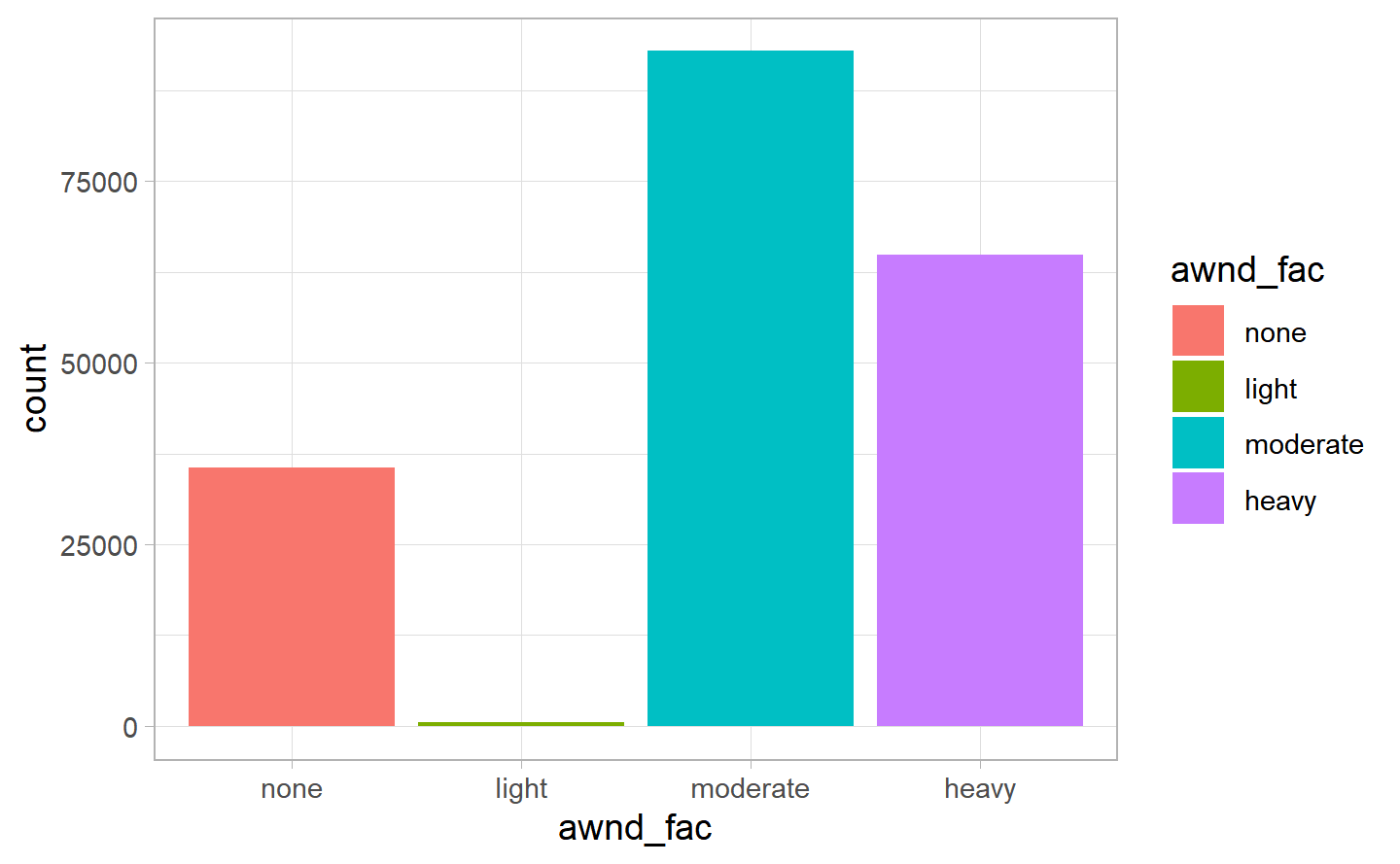
No dangerous wind speed is found, since the max has been 12.75 mph, and the wind starts to become dangerous at 74-95 mph (source). It has not even been threatening since it has been lower than 20 mph (source). We will create levels for the variables based on its quantiles. We have also created a variable based on the Saffir_simpson scale to show that our data has no threatening values for the average of wind speed, which takes all the values equal to No_Danger. Morover, the majority of days seem to have had “moderate” wind, which is quite interesting and it confirms that New York City is indeed a windy place, followed by heavy and eventually none. Only a few days have had light wind.
4.2.1.4 Weather Condition Variable(wt01)
Now we explore the wt01 variable, which has as definition a weather with fog, ice fog, or freezing fog (it may include heavy fog). If the value of the dummy is equal to 1, it means that during that day there has been this type of weather, if it takes value 0, on the other hand, it means that the weather was in different conditions. As already explained, we decided to take into account this type of weather, since we believe it could be the one having a higher correlation with the probability of a car crash, with respect to the other types of weather, since the driving conditions would not be optimal.
#> `summarise()` ungrouping output (override with `.groups` argument)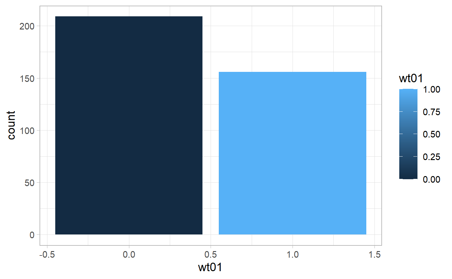
As we can see, there has been slightly more day without wt01 type of weather, even though we can find quite a lot of days with a positive value for the detection of this kind of weather.
4.2.1.5 Rain (prcp)
Eventually, let’s look at the prcp variable. This variable describes the inches of rainfall per day. Hence, if it takes value of 0, it means that it has not rained on that day, while, if it positive, it gives how much it had rained. We have already seen beforehand (figure ??) that the majority of days were giving a value of 0 for the rainfall, meaning that there has been no precipitation for the majority of days throuhgout the year. We could see that the major rainfall has been in december, followed by May, June and October.
#> `stat_bin()` using `bins = 30`. Pick better value with `binwidth`.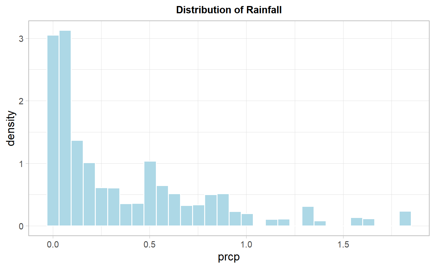
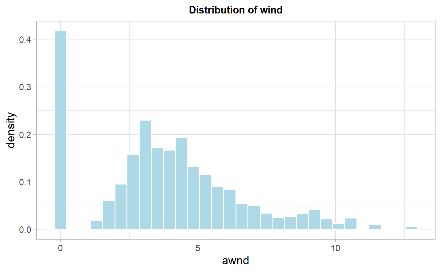
If we look at the distribution of the rainfall variables, without taking into account the observations with value of 0, since we want to be able to see if there are any other mode in the distribution, we can see that in general, as one could imagine, the rainfall takes quite low values in New York, with a maximum of 1.83 inches in a day.
#> `summarise()` regrouping output by 'date' (override with `.groups` argument)
#> `summarise()` ungrouping output (override with `.groups` argument)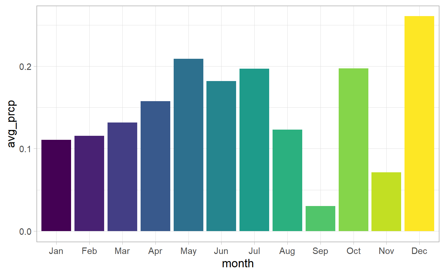
Moving on from the categories, we can look at the rainy days where there have been 148. The values or rain have a range of 0, 1.83. As we can see from the graph, throuhgout the year there is some variation. We can see an increase trend towards spring and a drop at the end of the summer, in September, which registers the lowest value of the year.
We will also define certain categories for the rainway fall coming from this website, which describes rainfall in the following way: > Rainfall rate is generally described as light, moderate or heavy. > * Light rainfall is considered less than 0.10 inches of rain per hour. > * Moderate rainfall measures 0.10 to 0.30 inches of rain per hour. > * Heavy rainfall is more than 0.30 inches of rain per hour.
4.2.1.5.1 Levels of Rain & number of accidents
| prcp | n_accidents |
|---|---|
| 0.00 | 113,996 |
| 0.01 | 7,643 |
| 0.04 | 5,351 |
| 0.02 | 4,098 |
| 0.11 | 3,585 |
| 0.03 | 3,549 |
| 0.06 | 3,431 |
| 0.08 | 2,820 |
| 0.07 | 2,609 |
| 0.20 | 2,231 |
| 0.10 | 2,107 |
| 0.48 | 1,897 |
| 0.53 | 1,812 |
| 0.54 | 1,778 |
| 0.17 | 1,754 |
| 0.79 | 1,266 |
| 0.75 | 1,208 |
| 0.45 | 1,195 |
| 0.90 | 1,124 |
| 0.57 | 1,091 |
| 0.86 | 1,088 |
| 0.26 | 1,074 |
| 0.24 | 1,029 |
| 0.70 | 990 |
| 0.30 | 972 |
| 0.62 | 932 |
| 0.29 | 907 |
| 0.09 | 894 |
| 0.81 | 694 |
| 1.57 | 680 |
| 0.68 | 663 |
| 0.63 | 639 |
| 0.23 | 626 |
| 0.34 | 626 |
| 0.42 | 626 |
| 0.39 | 615 |
| 0.37 | 611 |
| 1.83 | 609 |
| 0.96 | 608 |
| 0.13 | 596 |
| 1.66 | 589 |
| 0.51 | 582 |
| 1.82 | 581 |
| 0.12 | 576 |
| 0.18 | 576 |
| 0.60 | 571 |
| 1.18 | 560 |
| 0.36 | 558 |
| 0.95 | 555 |
| 0.80 | 553 |
| 0.05 | 552 |
| 1.32 | 549 |
| 1.33 | 549 |
| 0.32 | 543 |
| 1.01 | 535 |
| 1.16 | 531 |
| 0.21 | 522 |
| 0.74 | 491 |
| 1.31 | 487 |
| 0.52 | 477 |
| 1.03 | 464 |
| 0.64 | 439 |
| 1.38 | 424 |
| 0.50 | 418 |
| 0.88 | 377 |
| 0.58 | 362 |
| 0.25 | 352 |
4.2.1.5.2 Summary Statistics of Rain
| summary Metric | value |
|---|---|
| Min. | 0.010 |
| 1st Qu. | 0.040 |
| Median | 0.180 |
| Mean | 0.365 |
| 3rd Qu. | 0.570 |
| Max. | 1.830 |
4.2.1.5.3 Correlation of Rain and other variables
| other_variables | prcp |
|---|---|
| wt01 | 0.51 |
| snow | 0.12 |
| awnd | 0.11 |
| pedestrians_injured | 0.03 |
| snwd | 0.03 |
| day | 0.03 |
| monthday | 0.03 |
| multiple_cars | -0.02 |
| persons_injured | 0.01 |
| cyclist_injured | -0.01 |
| hour | 0.01 |
| latitude | 0.00 |
| longitude | 0.00 |
| persons_killed | 0.00 |
| pedestrians_killed | 0.00 |
| cyclist_killed | 0.00 |
| motorist_injured | 0.00 |
| motorist_killed | 0.00 |
| postvz_sl | 0.00 |
There are 67 different levels of inches of rainfall in our dataset. Without considering the zero value observation, the mean of the variable is at 0.36, the median at 0.18 and the 1st and 3rd quantiles are respectivels at 0.04 and 0.57, so the values are fairly low.
The variable is mostly correlated with wt01 (50%), and also with snow, awnd and snwd, but it’s always below 15%. Which makes sense, since we have already mentioned these correltaions in our analysis of the previous variables (awnd, snow and snwd).
As already mentioned, we have created a factorial variable based on information we have found online. Following, we analyse more this new factor.
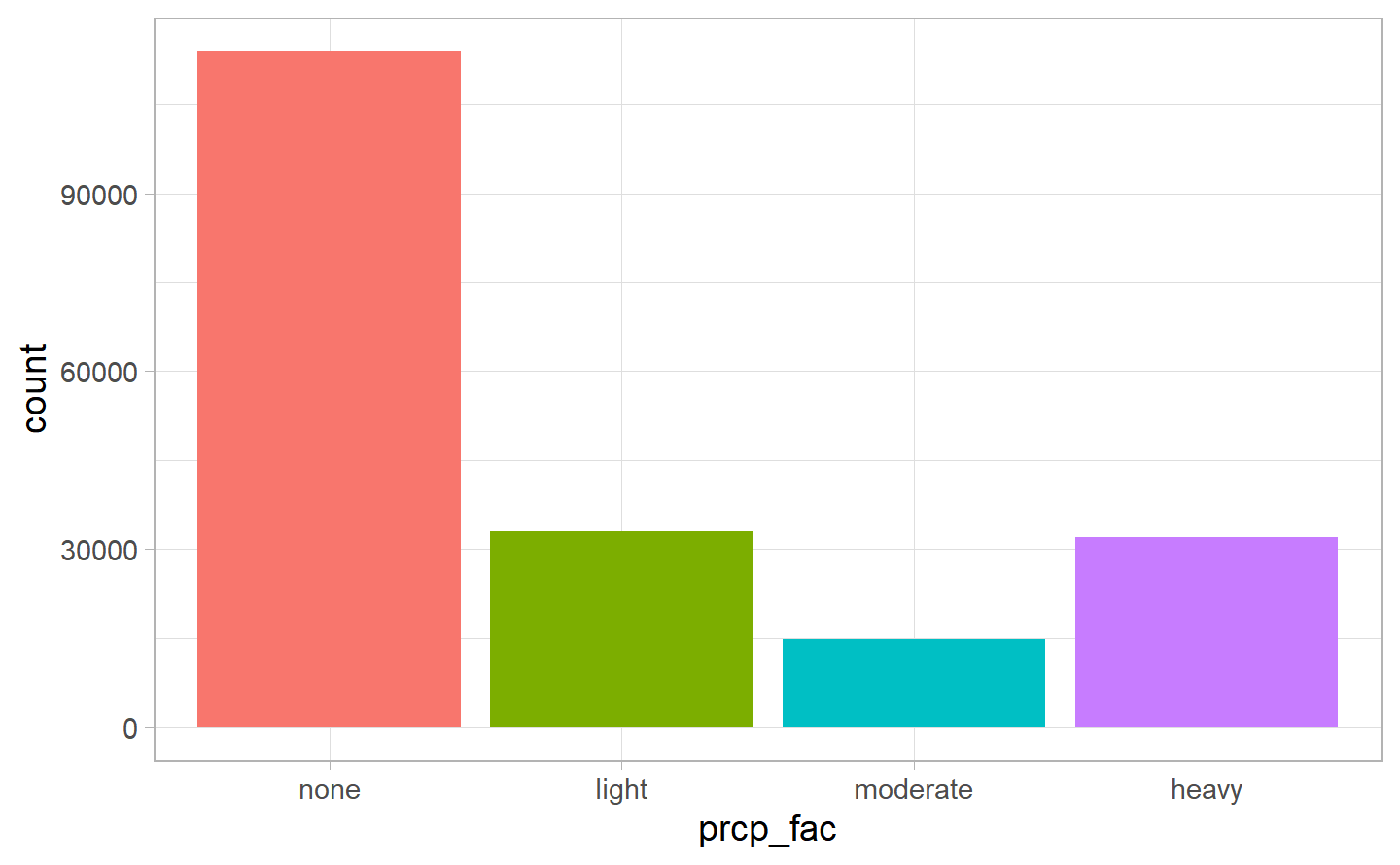
As we can see, the majority of the values take a “none” level, since the majority of the days in our dataset was without rain (value of prcp = 0). Interestingly enough is the fact that there are more “heavy” rain days than “moderate” ones, with respect to the levels we have created.
4.2.1.6 Relationship between all weather variables
| var | snwd_fac | snow_fac | awnd_fac | prcp_fac |
|---|---|---|---|---|
| snwd_fac | 1.000 | 0.552 | -0.270 | 0.095 |
| snow_fac | 0.552 | 1.000 | -0.230 | 0.231 |
| awnd_fac | -0.270 | -0.230 | 1.000 | 0.058 |
| prcp_fac | 0.095 | 0.231 | 0.058 | 1.000 |
Afterwards, we calculated the new correlation, and we can see that the factor variables we have created have a high correlation among them, especially for the snow and snwd factor is almost 100%, while the factor variables for rain is correlated, but only at 20% with the others. The weather is highly correlated to the precipitation and at 20% with the snow and wind factor variables.
Conclusion of this EDA: ** Due to the high correlation between the two snow variables, we have decided to use only one of them. We will keep only one variable for the snow (snow_fac) and one drop the other one (snwd_fac). Moreover, we have decided to drop the WT01 variables, as it is too general, and we want to have clear and straightforward analysis of our modelling.**
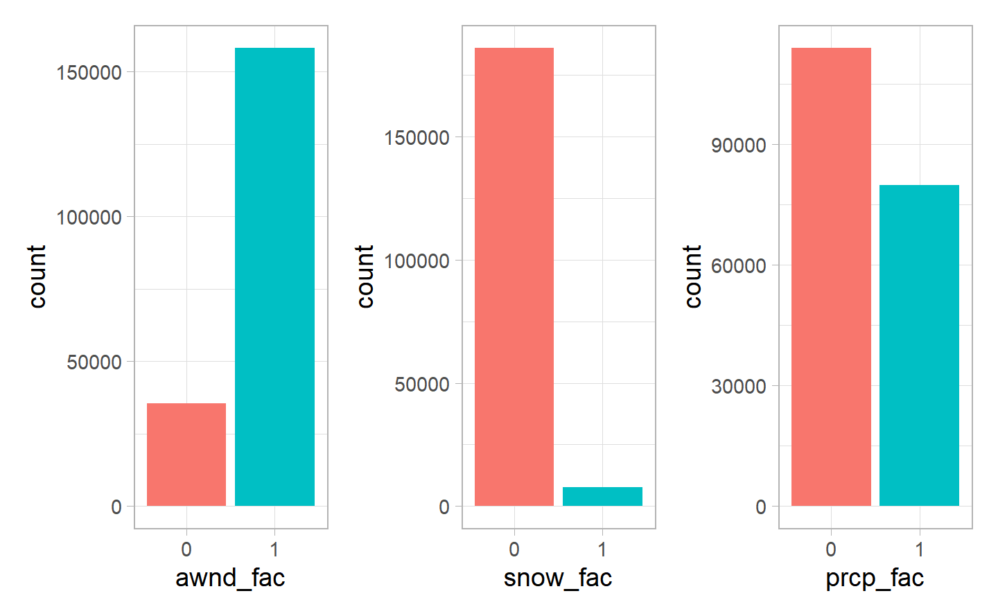
We decided to include also an alternative to the factor variables, which is creating a dummy for each factor (wind, snow and rain). Following, the creation of such variables, which we will use in the modelling chapter.
4.3 Multiple car accidents in different weather conditions
We will look at how the accidents have developed for single and multiple cars under different weather conditions. On the y-axis we will always see the chance of accident involving injury and on the x-axis the type of the accident.
4.3.1 Rain
First, we look at the proportion of accidents by their category.
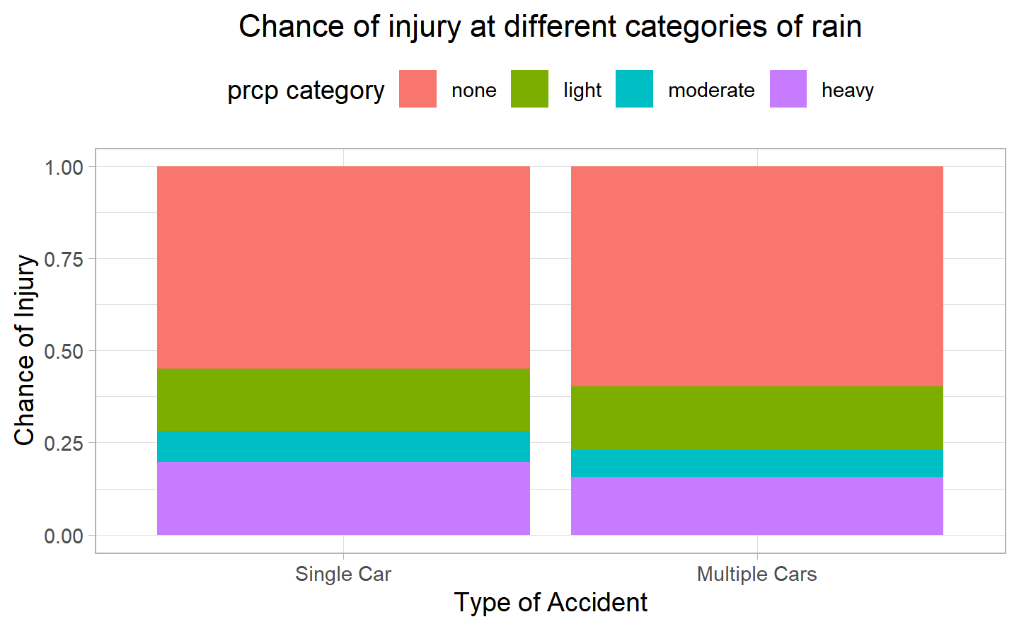
What can be observed here is that the proportion of the accidents in the none category of the rainfalls is slightly larger for multiple cars, while single car accidents are impacted more by heavy rain.
4.3.2 Average wind speed
Next, we can see a clearer picture for the average wind speeds.
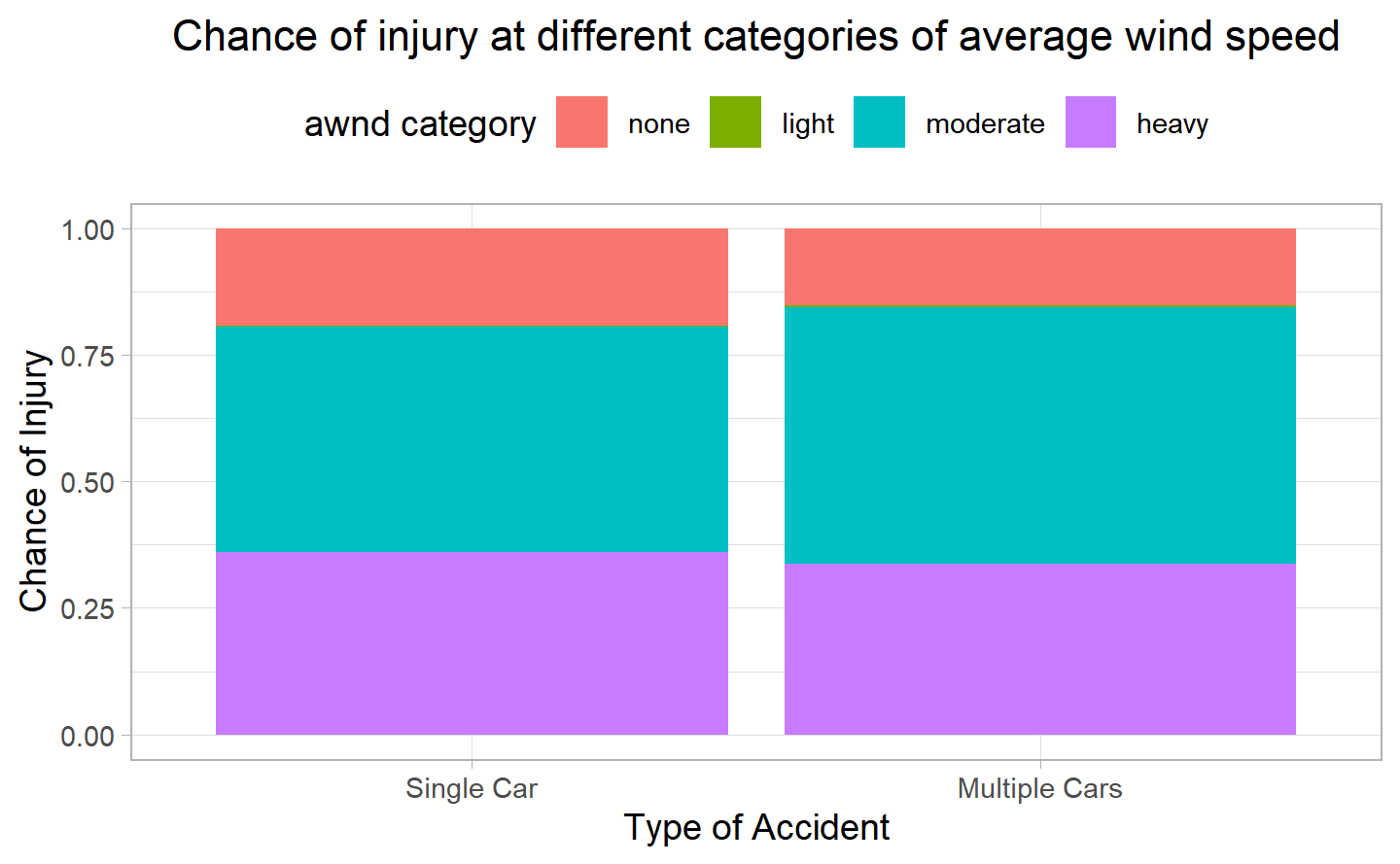
Most of the accidents happen at the moderate wind speed followed by high wind, this goes along with the previous observation of NYC being a windy city. However, it is interesting to see that a low wind speed plays no role for either of the two categories and that the impact of days without any wind in multiple car accidents is lower than single-car ones.
4.3.3 Snowfall
Eventually, we can look at the snowfall.
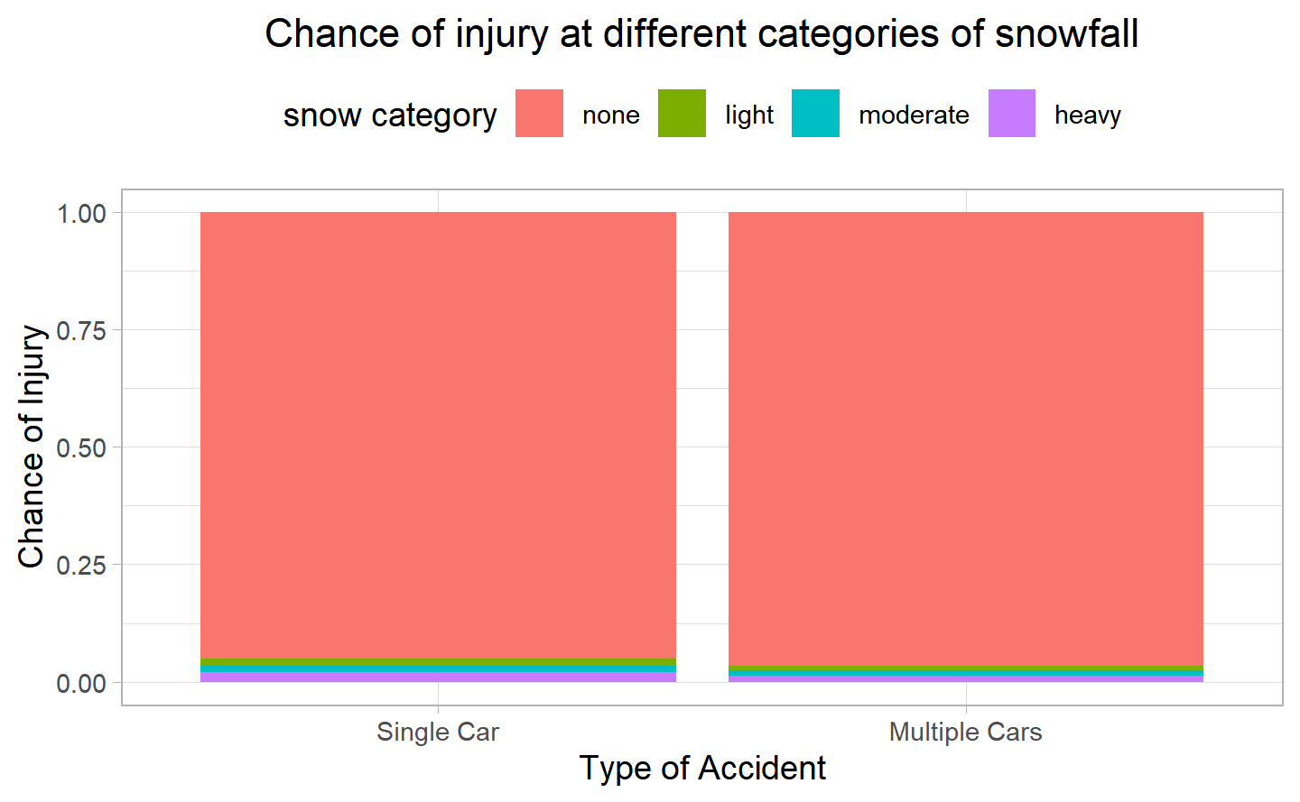
Here we can clearly see that, as there were not many instances in which there were positive snow, this proportion if very small for both categories but even smaller for multiple cars.