5 Variable Selection

After having analyzed the weather trends, in this section, we identify the most important contributing factors, which represent the reasons why an accident happens only given the information from the collision dataset (therefore excluding weather and the speed limits). It has to be noted that this is done solely for exploration purposes, as we have too many contributing factors, which makes analyzing all of them unfeasible. The variables selected will then be used for exploring both the collision data, as well as accidents at different speed limits, while for the modelling part of the analysis the whole dataset will be used, as we will consider also the other ones (i.e.:the weather and the speed limit) and the interaction between the different features could change the importance of the variables, due to the correlations among them.

First, we will construct a general correlation plot and then we will look at accidents that have caused an injury or fatality using a lasso regression and a random forest.

Note: Please do note that although we have used some modelling approaches, this is not our modelling section and we do not consider many aspects of modelling control, such as training and testing, balancing the data and model diagnostics. Once again, these methods are only used for an initial variable selection and to identify possible interesting relationships that deserve their own visualizations.

We will first create a variable for this section which will only contain the contributing factor as the independent variable and the maximum between injury or death as the response variable. We will also take the categorical variables of the rain from the last chapter and use them again.

5.1 Correlation plot

A good initial way to get an idea about the relationships is to create a custom correlation plot where the absolute significance (in our case above 0.19) are identified. As a normal corrplot would be unsuitable to display all our variables, we will create a function for a more customized one. Please do note that none of these correlation plots is symmetric.

The function can be found below.

In the first case, we will treat the weather factors as categorical variables and then we will look at them by day with the help of the dummy variables we have created previously. This means that for instance if the rain on a given day is above zero, then we put a 1 for that day to identify it as a rainy day. We do the same for windy and snowy days.

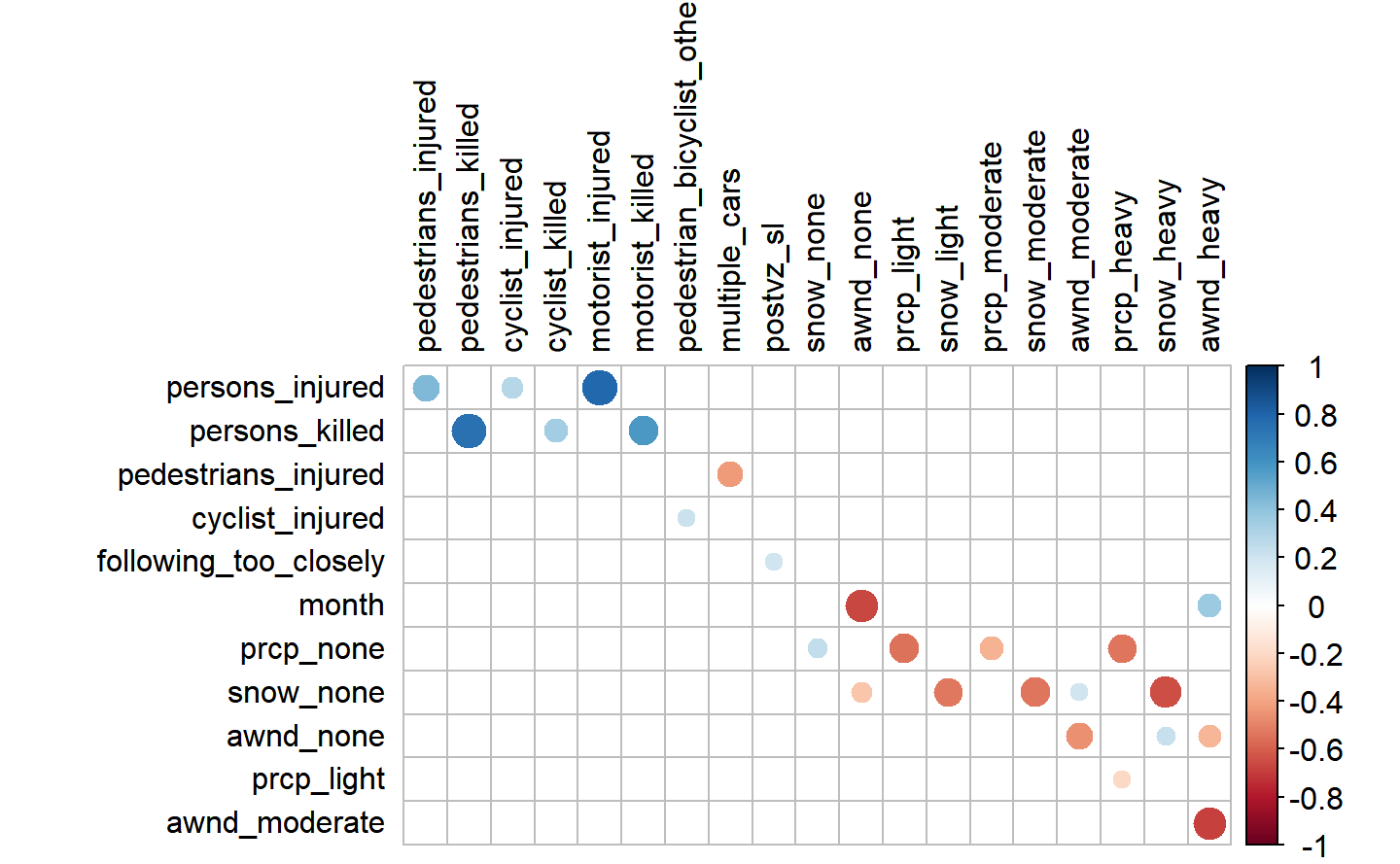
We can see that if multiple cars are involved, it probably means that pedestrians were not injured, which is straightforward, since if there are more cars involved, the victims were most probably inside one of them, rather than being in the street. Another observation that can be made is that the “closely” variable, which represents “following_too_closely” as a contributing factor, seems to be somehow correlated (around 0.2) with the speed limits (“postvz_sl”).

The variable pedestrian_bicylist_other may be more specific for cyclist, as we can see a positive correlation between the two, However, it is interesting not seeing any correlation with pedestrians injuries or deaths.

Many of the weather data features correlate among each other, as we could already see before, however, they do not seem to have any relationships with the variables coming from the other dataframes, at least at this point. Furthermore we can see that the average wind speed (awnd) is correlating with the month variable, which is in line with the increasing trend we have seen in the eda analysis.

The remaining relationships are between persons injuries or deaths, as well injury or death of other road users (i.e pedestrians and etc), which were already previously mentioned as they were used to create the aggregated variables for total injuries and deaths.

Now we can look at the weather by day, in the sense that we look at the day in which the variables were postive.

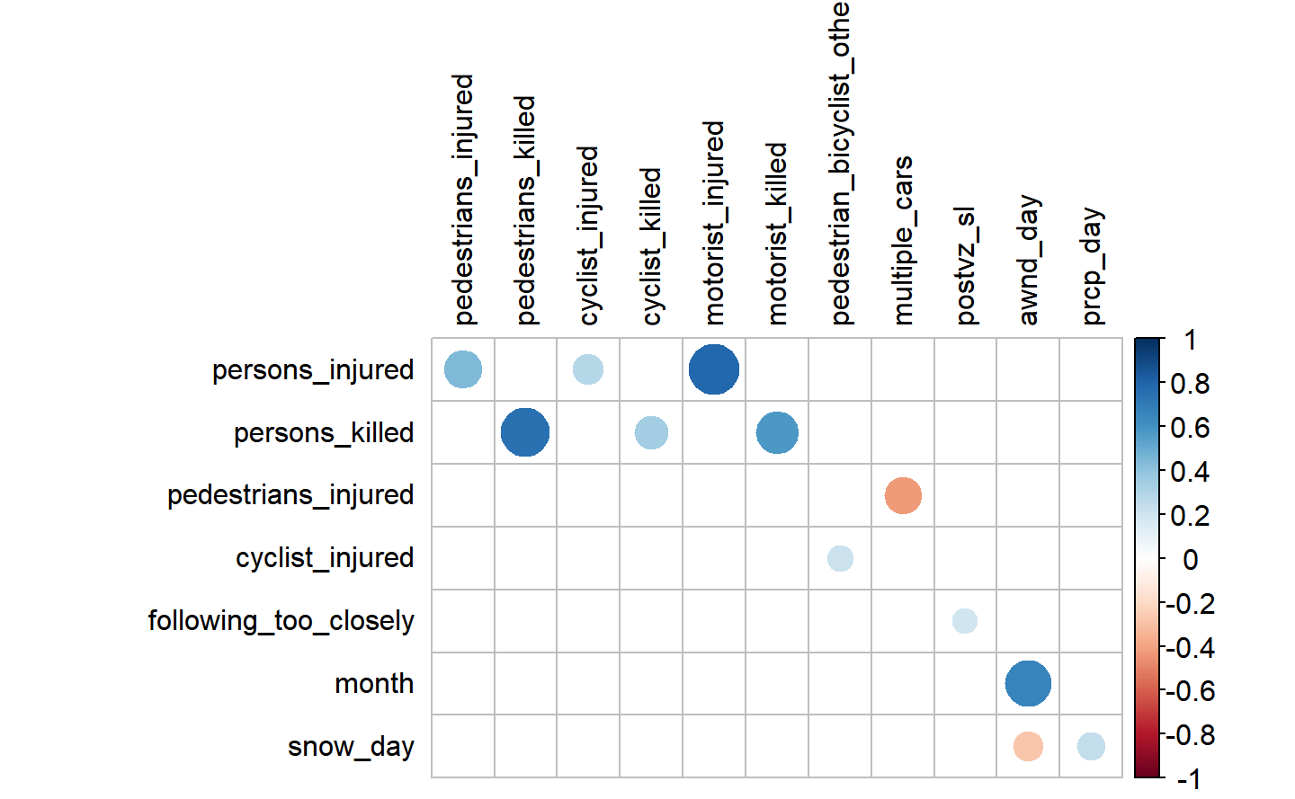
Besides the interactions between the weather variables we have observed previously, we do not see anything new here. We also have the wind by day still varying largely by months meaning that going towards the last months of the year we have higher wind speed, however we do not have to take into account that we have some missing data for the first 69 days, having the first value only from mid March, but it seems to get windier as the year progresses. The details of this variable can be found in the wind analysis of the previous chapter.

5.2 Preparation for selection

Before proceeding to the selection of the most important contributing factors, in the selected dataset with only the contributing factors we will create a new column called injury_death, which represents the accident having caused an injury or death. This variable will be the basis for our selection with the aformentioned models.

Then we can proceed with our two models, by starting with the lasso regression.

5.3 Lasso Regression

To have interpretability and choosing among many contributing factors (excluding the weather conditions, speed limits and all the other features), we will use Lasso (l1) regression. Our response variable is the aformentioned injury_death which shows whether there has been an injury or a fatality. We do not have many instances where there was death (only 221), but do have 41438 instances in which at least one person was injured.

At this stage (EDA), we will not have a train/test approach for two reasons: firstly, our aim at this point is not training a predictive model, but rather using a regression model to find a pattern in the data and only selecting the most important contributing factors to focus on; secondly, the lasso regression and regularization help overcome problems of complexity and overfitting and this method brings simplicity to our analysis. Nevertheless, later on, we have also used the same modelling approach, but this time with a penalty.factor from the glment package (Friedman et al. 2020) to control for the variables ignored at this stage (namely the weather and speed limits). However, due to the complexity of the model and the huge computational time, altogether with the multiple errors that have incurred, our final decision was to move towards another model. The lasso process, though, can be found in the appendix, while in the modelling we can find the process used.

As mentioned previously, we will make use of the (Friedman et al. 2020) in order to proceed with our analysis. The reason why we were convinced by this model is that it is a good way to select the variables, as it forces the coefficients of some variables to be exactly equal to zero, while it will keep only the most significant ones. The process is based on a penalty imposed to the linear regression in the case in which there are too many variables. The purpose is to balance accuracy and simplicity. We think is a good choice as it will lead us to have a lower number of variables and it will hence be easier to interpret them and to analyse in detail only the most improtant ones, since, especially with regards to the contributing factors, the number of variables present in this dataframe is quite high. The biggest limit of this process, though, is the fact that if there are grouped variables, hence being highly correlate among each other, the model does not perform as well. An example of this method’s implementation can be found here.)

Table 5.1: Performance of different lasso models
term	model _min	model _1se	model _3var
variables	46	23	3
accuracy	0.79	0.79	0.79
kappa	0.04	0.04	0
sensitivity	1	1	1
specificity	0.03	0.03	0
pos_pred_value	0.79	0.79	0.79
neg_pred_value	0.72	0.75	NaN
precision	0.79	0.79	0.79
recall	1	1	1
f1	0.88	0.88	0.88
prevalence	0.79	0.79	0.79
detection_rate	0.78	0.78	0.79
detection_prevalence	0.99	0.99	1
balanced_accuracy	0.51	0.51	0.5

Three models were created: one having the minimal lambda that was found using a cross-validation (model_lasso_min), one having lambda within one standard error (model_lasso_1se) and one having the lambda corresponding to the model that would select three variables (model_lasso_3var). \[(𝑌−𝑋1𝛽1−𝑋2𝛽2−...)2+𝛼∑𝑖𝛽𝑖|\]

Looking at the formula for lasso regression, we can see that, as the penalization $𝛼$ increases $ ∑|𝛽𝑖|$ is pulled towards zero, with the less important parameters being pulled to zero earlier in the process. At some level of 𝛼, all the 𝛽𝑖 have been pulled to the plot,which shows that variables with postive coefficents, such as pedestrian_bicyclist_other, indicated in dark blue, failure_to_yield indicated in light green and traffic_control_disregarded in pink, are forced to be equal to zero at the very end, and negative coefficents, such as passing_too_closely backing_unsafely, are being selected out as last. At some level of 𝛼, all the 𝛽𝑖 , meaning our contributing coefficents, are pulled to zero.

Please note that here interpretating the coefficents makes sense, as we are looking at standardized variables (they are all binary).

We proceed by fitting the models and finding their coefficients, that we will use to get the predictions given by them. Which will make us able to assess the quality of the different models, by looking at their confusion matrices, that can be found in the tables above. Comparing them, we can see that the model within 1se is the simplest and yet the most predictive one (having the highest pos_pred_value and neg_pred_value) and, although deceitfully, it may seems that the absolute accuracy is high in all cases, equal to 0.79 for the three models. However, the balanced accuracy is in fact around 0.51 for the first two models, which means they are not doing a much better job than using a random model, while the third one’s predictions are the same as choosing randomly one of the two levels, being the accuracy exactly at 0.5. The models already indicate that contributing factors are not very important in the modelling of injuries or deaths, however we will still consider them by following more in-depth model construction in our last chapter. Please do note that here having no injuries nor fatalities is the positive class and it is serving as our reference.

To have an idea of what would be the most important three variables selected by the lasso for our eda, we have to look at the next table.

Table 5.2: The three most important variables from lasso regression
term	estimate
(Intercept)	-1.317
failure_to_yield	0.225
pedestrian_bicyclist_other	0.576
passing_too_closely	-0.050

We can see that pedestrian_bicyclist_other which represents the error or confusion of the pedestrian or the bicyclist has the highest absolute coefficient and hence could be considered the most important variables among all, given that all our variables are binaries and hence the coefficients could be interpreted as the increase of probability of having an injury or a fatality in a given accident.

5.4 Random Forest

Random forest is less prone to overfitting than many other algorithms, hence why it is suitable for finding patterns in our data without a training and testing subsets.

#> Confusion Matrix and Statistics
#> 
#>           Reference
#> Prediction      0      1
#>          0 151780  40356
#>          1    406   1255
#>                                         
#>                Accuracy : 0.79          
#>                  95% CI : (0.788, 0.791)
#>     No Information Rate : 0.785         
#>     P-Value [Acc > NIR] : 1.27e-06      
#>                                         
#>                   Kappa : 0.042         
#>                                         
#>  Mcnemar's Test P-Value : < 2e-16       
#>                                         
#>             Sensitivity : 0.9973        
#>             Specificity : 0.0302        
#>          Pos Pred Value : 0.7900        
#>          Neg Pred Value : 0.7556        
#>              Prevalence : 0.7853        
#>          Detection Rate : 0.7832        
#>    Detection Prevalence : 0.9914        
#>       Balanced Accuracy : 0.5137        
#>                                         
#>        'Positive' Class : 0             
#>

Moreover, we have decided to run a random forest model since it allows us to have a clear idea about the importance of each variable and see if there is any strong correlation between the variable we want to predict (hence the injury_death variable previously created) and the other explanatory variables. In our case, we want to have a classifier predictions, with the results telling us if there will be an injury or a fatality (having prediciton taking value equal to 1), or not (taking value equal to 0). In order to do it, we have to transform our variables into factors, otherwise the model will treat them like numbers and not like levels. Once we have done that, we can run the model, which takes a couple of hours before it is completely computed, this is why we decided to store the result and load it, instead of running the code each time. Once it is ready, we will use it to make the predicitons to see if the model is a good fit for our analyisis. We can see that the accuracy is almost 80%, which is fairly good, and that it has an almost perfect sensitivity (this is due to the fact that there are way more observations taking the value of 0, rather than 1, the dataset is hence unbalanced), while on the other hand the speificity is very very low.

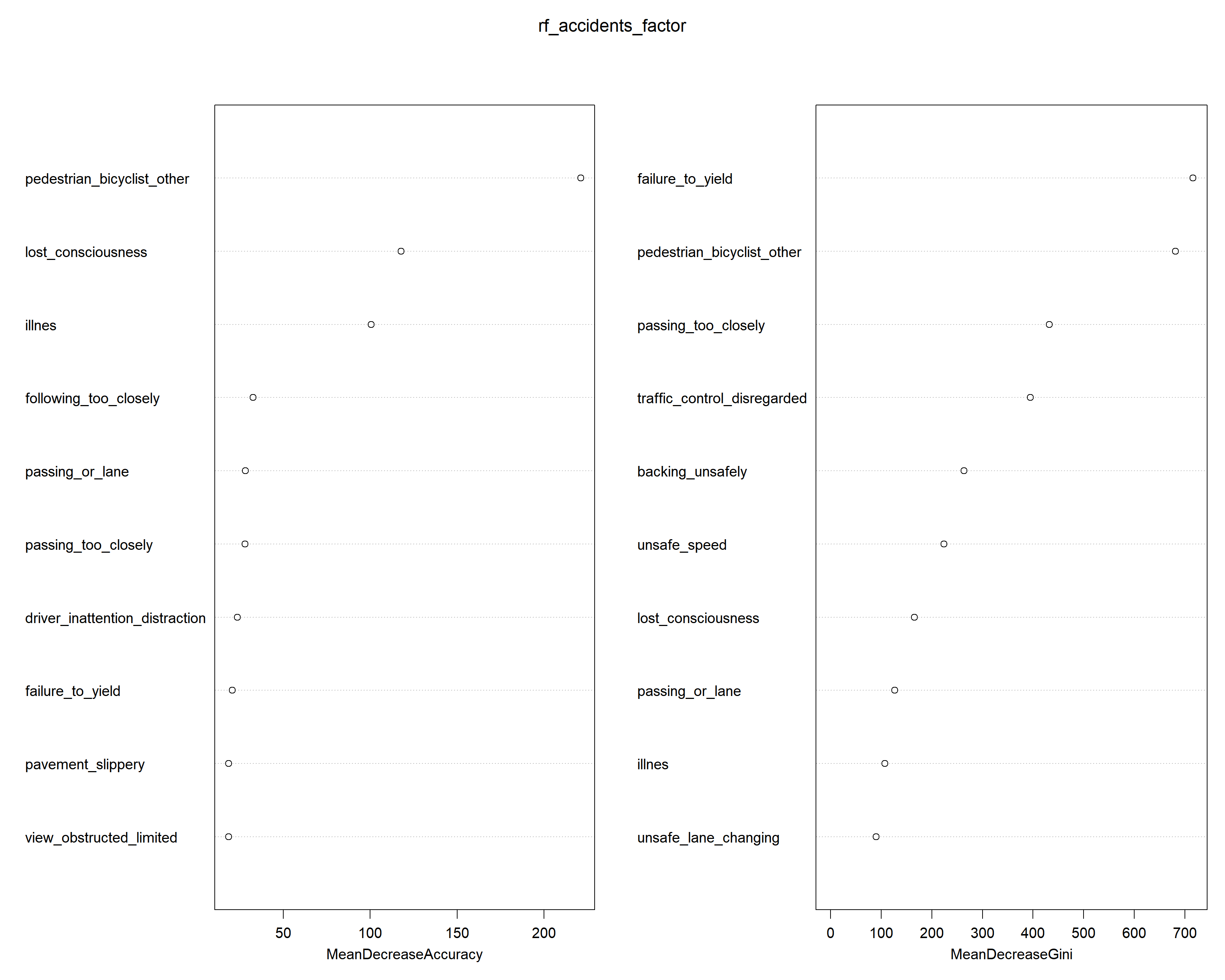
Looking at the importance of the variables, in terms if MSE are pedestrian_bicyclist_other, lost_consciousness and illness. The MSE is the Mean Square Error, being the mean of the difference between the predictions given by the model and the real observations, to the square.

\[\text{MSE} = \displaystyle \frac{\sum_{i}^{n} ((Y{i} - \hat{Y})^2)}{n}\]

It is a good method to detect the goodness of fit of a model, since it score the value of the error being how much the prediciton of the model is different by the value is trying to predict. On the other hand, for the Gini Impurity the most important variables are failure_to_yield for right of the way and pedestrian_bicyclist_other, passing_too_closely, traffic_control_disregarded, backing_unsafely and unsafe_speed as we can see from our graph. The Gini Impurity of a node is the probability that a randomly chosen sample in a node would be incorrectly labeled if it was labeled by the distribution of samples in the node, so, for node n it is 1 minus the sum over all the classes J (here J = 2) of the fraction of examples in each class p_i squared. (source)

5.5 Final Decision

Considering the outputs from the correlation matrix, the lasso regression as well as the random forest, it is worth looking at the following contributing factors:

pedestrian_bicylist_other with injuries at different speed limits proposed both by lasso regression and random forest;
Having to chose between following_too_closely proposed by the correlation plot (correlating with postvz_sl) and passing_too_closely which is put forward by the lasso regression and random forest (correlating with injury_or_death) we will choose the former, as it makes more sense to look in the context of speed limits and see what is happening when the cars folllow each other with a too short distance, which is what is causing an accident;
Lastly, we will look at the unsafe_speed, which makes sense in the context of speed limits and it also proposed by the random forest and also one of the top 5 lasso regression coefficents not displayed by our table.

References

Friedman, Jerome, Trevor Hastie, Rob Tibshirani, Balasubramanian Narasimhan, Kenneth Tay, and Noah Simon. 2020. Glmnet: Lasso and Elastic-Net Regularized Generalized Linear Models. https://CRAN.R-project.org/package=glmnet.